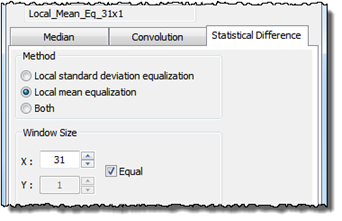
The statistical differencing dialog offers two ways to enhance the contrast:
- Local Standard Deviation equalization.
Either one or both methods can be performed on the data set.
This method simply subtracts the mean value of the nearest neighbor pixels within the filter window:

This is a powerful way to reduce long-range waves and image bow.
The Standard Deviation (SD) equalization scales the height values by a factor given by the SD of the global image, sg divided by the local standard deviation sl found in the filter window.

This way the local SD and contrast will appear the same all over the image.
When “Both” is checked both Local Mean and Local Standard Deviation equalization will be performed.
The filter window, i.e., the number of pixels used for calculation of the local mean and SD values is defined by the X, Y filter kernel Size parameters. To have the desired effect the kernel size should be chosen so that it is larger than the size of the features being studied, but smaller than the long range structure, which should be suppressed.
When the equal check box is set, the X and Y kernel size parameters will be set equal when using the up down buttons.
The auto apply button can be checked so that every modification of the filter settings will cause the filter to process immediately so that the effect can be monitored simultaneously. Otherwise clicking on the Apply button will apply the currently defined filter.
The auto apply function is a good way to interactively define the filter that gives the best result. However, for larger kernels the response time may be so long that it is more practical to turn off this feature.
Below is seen an example of an image filtered by the Statistical Differencing filters:

Statistical Difference filtering example: The top image is the original unfiltered image. The second image has been subtracted by the local standard deviation values using a 45x45 window size. The third image has been subtracted by the local mean values. The last image has been subtracted by both the local SD and local mean values. All results have been using a 45x45 window size. It is seen that in this case the "Local Mean Equalization" results in the best contrast and it is therefore suitable as a preprocess for particle analysis.