
A force volume image consists of an equidistant grid of force curves. For an introduction to force curves and the used terminology please see the Force Curve Analysis section in this manual. The Force Volume curves can be other than deflection vs. height, e.g. if the image is recorded in tapping mode it could be amplitude or phase. In the following deflection is assumed. The force volume image may be recorded simultaneously with a height image of the same or different resolution. The force curves may be recorded with a force trigger at an absolute deflection level or a deflection level acting relative to the baseline. It is important to be aware exactly how the force volume image has been recorded in order to make full use of the powerful Force-Volume features in SPIP™.
When a Force Volume image is loaded at set of dedicated tool will be available in the ribbon.
Most of the tools in the General tab are generic and identical with the tools found on the General tab of 2D Images, including Color Scale adjustments, zooming etc. Therefore, only tools dedicated to Force Volume are described here.
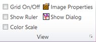
This panel contains the same functions as for 2D images, but in addition also an option, Grid On/Off, for having a grid overlaid onto the force volume image highlighting the pixel boundaries and a button, Show Dialog, for displaying the force curve analysis dialog, which contains various processing settings shared with the force volume image analysis.

To extract and show the force curve recorded in at a specific pixel point use the Select Curves tool key. The selected curves will all be shown in the same force curve window, which can be viewed in Analysis or Comparison view mode. If Auto Preview is checked on in the Force Curve Dialog the Force vs. Separation curve will automatically be calculated whenever a new force curve (deflection vs. height) is selected. Once selected, force curves at other positions can be shown by dragging the selection marker. Different colors are used to distinguish between the selected force curves. The pixel coordinates of the cross is shown in the title bar of the force curve window.
It is also possible to calculate an average force curve within an area by using this tool for drawing a box.

When this button is enabled, the force curve markers in the selected force volume image will also be displayed in any 2D images associated with the force volume image. The markers can be moved and deleted in the 2D images, and the original markers in the force volume image will follow. In order to remove the force curve markers from the 2D images, select the force volume image again and toggle the Synchronize Markers button.
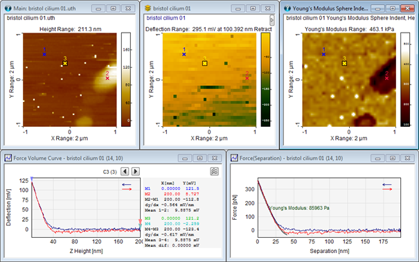
In this example three markers are synchronized to same lateral position for the topographic, the force volume and the deduced Young's modulus images. The graphs deduced from marker 1 is shown a the bottom.
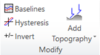
Click this tool key to baseline correct all curves in the force volume image using the settings of the Force Curve Dialog.
Click this tool key to hysteresis correct all curves in the force volume image.
Invert the image by changing the sign of the values.

In several force volume image formats all force curves starts at the Height = 0. For analyzing adsorbents, e.g. bio-molecules, this is perfect. But for analyzing surface topography this is not desirable. One type of analysis is for example to calculate the point where the tip and surface first touch and generate an image from these points, or for calculating a height image at a deflection point lower than the one used during acquisition. In order to facilitate this SPIP™ offers the option to offset the height of all force curves in the force volume image using the heights from a topographic image. When clicking the “Add Topography” button SPIP™ shows a list of height images related to the Force volume image. Select one of the images in the list to have it added to the force volume curves height axes. Select “No Topography” in order to get back to the original data.
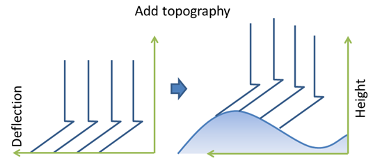
Illustration on how the force curves are offset by topographic height values when the Add Topography is applied.
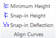
For comparing curves and perform calculation it is often an advantage to have the curves aligned. Here we provide two alignment methods:
Click this button in order to align all curves in the force volume image to start at the same minimum height.
Click this tool key to align all curves in the force volume image to have the same snap-in deflection value.
Click this tool key to align all curves in the force volume image to have the same snap-in height value.
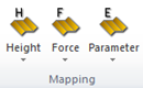
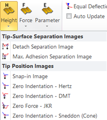
From force volume images new images can be mapped based on detected height and force values or calculated parameters.
In SPIP™ by the “tip position” we mean the vertical position of the tip apex. The tip position is the sum of the (sensored) height of the Z piezo and the deflection of the cantilever. “Tip position” differs from “separation” by not being offset to zero at maximum indentation: In the Force vs Separation curves the left most point is always forced to have Separation = 0.
Mapping Separation is useful for studying adsorbents in a comparably hard surface, e.g., the rupture of bonds inside or between biological molecules, or polymers in general, including unfolding. On a hard surface using a soft cantilever the indentation is typically negligible and the force-separation curve is vertical at zero-separation. Hence, when pulling molecules with the AFM tip, then Separation directly gives the pulling distance.
Mapping Tip Position is useful for gaining information related to the topography of the surface, for example for mapping the point where the tip is not deforming the surface.

The Detach Separation Image will contain the separation values at the detected detach points on the retraction curves (deflection vs. height curves). Note that it is the separation which is mapped and not the height meaning that this is a map of maximum tip-sample separation before detachment/rupture. So in case of a polymer/protein/DNA-chain covered surface this will be a map of the pulling lengths.

Going hand in hand with the Maximum Adhesion Force map this is a map of the corresponding separation points. This is most interesting when the adhesion is caused by molecules which will stretch before bond breaking. Then it is possible to get a map of the molecule lengths when the strongest bond is yielding. This can for example be used for investigating which binding sites is used for binding a specific molecule either to the surface or to the tip.
As the search range for point of maximum adhesion can be restricted on the Pulling tab in the Force Curve Analysis Dialog it is possible to address selected events in the retract force curve, not always just looking at the global maximum adhesion point.

If present this is the tip position after long or short range attractive force gradient has overcome the cantilever spring constant and has pulled the tip to the surface. This point is a balance between repulsive surface forces, the attractive tip-surface forces and the cantilever retract force. Hence, a soft surface will be indented slightly at this point. If snap-in is present in all force curves SPIP™ can create the snap-in tip position map, giving a good estimate of the unperturbed surface. Note, that if "Align Snap-in Heights" has been performed the image will be flat.

In SPIP™ the Point of Zero Indentation for these two models is the tip position where the tip touches the surface without actually indenting the surface; thus the applied force is zero. Mapping this point yields an image of the undisturbed surface not deformed (indented) by the tip. Note, that the method for identifying this point is an option in the Force Curve Analysis dialog.
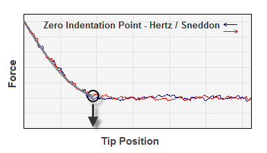
Tip position deduced by fitting a Hertz model to the force curves.
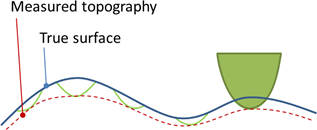
A sketch showing the measured surface height along with the true surface height

In SPIP™ the Point of Zero Indentation in the DMT models is the tip position where the retraction forces exerted by the cantilever balance the attractive forces between the tip and the surface. This point is found on the retract force curve where adhesion is maximum. Typically the tip will pull off when the retraction force is increased further. If the tip and surface comply with the model, the tip apex will just exactly touch the surface at this point, and mapping this point will give an image of the undisturbed surface not deformed / indented by the tip. Note that the method for identifying this point is an option in the Force Curve Analysis dialog.
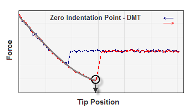
Tip position deduced by fitting a DMT indentation model to the force curves.

The two reference points used in the JKR model modulus calculation are the point of maximum adhesion and the zero force crossing, both on the retract curve.
The zero force crossing is where the adhesive and repulsive forces balance each other and the external force exerted by the cantilever is zero. The point of maximum adhesion (see DMT model above) is the point of the highest external force necessary for balancing the adhesive forces between tip and surface. The tip apex will be a little bit above the equilibrium height of the surface at this point.
The true zero indentation point is somewhere between these two points or if a snap-in point is present between the snap-in point and the Max. Adhesion point (Zero Indentation Point for DMT). Hence the Point of Zero Force tip position image is one qualified guess on the true undisturbed surface.
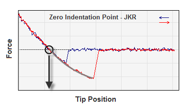
Tip position deduced by fitting a JKR indentation model to the force curves.

The Max Adhesion Image will contain the calculated force value at the detach points on the retraction curves. The largest negative deflections are converted to force using the spring constant entered in the Force Curve Analysis Dialog. The Max Pull Forces detected in the Force Volume Curves are reported as positive although they may appear as negative values in the Force vs. Separation plots (depending on the Set Attractive Forces Positive checkbox in the Force Curve dialog)
The Max Load Force Image will contain the maximum force values for all curves. If the Force Volume image has been recorded with an absolute force trigger the Max Load Force Image would be expected to be flat.
The Snap-in Force Image will contain the snap-in force values detected from all curves. The forces in the map are reported as positive though they will usually appear as negative value Force vs. Separation curves generated form the Force Volume Curves.
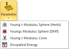
The Young's Modulus Images can be calculated based on the three supported models, Hertz hard-sphere-on-soft-flat-surface model, DMT indentation model and the Sneddon hard-cone-on-soft-flat-surface model. The settings on the Indentation tab in the Force Curve Analysis dialog are used for the fitting. It is important to define these settings including a realistic estimate for the tip radius of curvature and to execute a Baseline Correct for the entire Force Volume image before making this map. See details in the Force Curve Analysis section of this manual.
The following shows an example of a calculation of the Youngs' Modulus image:
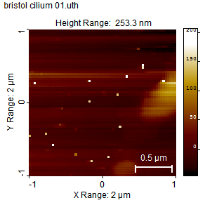

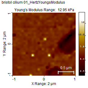
Calculation of the Young's modulus image: The left image shows the topographic image acquired simultaneously with the force volume image shown secondly. The third image is the calculated Young's modulus image where the Hertz model was used
The Dissipated Energy will contain the calculated dissipated energy for all curves.
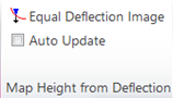
This function will at each pixel in the force volume image find the height value corresponding to the deflection value read out at the position of the active cursor (last moved) in the active force curve extracted using the force curve selection tool. If the active cursor is on the approach curves, then it is the approach curves which are searched for the chosen deflection value. If the active cursor is on the retract curve, ten it is the retract curves which are used.
The resulting image corresponds to a contact mode image recorded at a set point equal to the chosen deflection value.
Note, that not all force volume images will have the surface topography reflected in height axis of the force curves. In such cases all force curves will start at zero height. Use the “Add Topography” function for adding the topography from the corresponding height image to the data before calculating the Equal Deflection Image.
When this state button is set the Equal Deflection map will be updated automatically when the active marker is moved.
The Extract panel offers different ways of extracting data from the Force Volume image without modifying the data.
Use this function to duplicate the shown layer to a new image window. You can select the height layer by use of markers in the connected force curve window, see the Handling the Force Volume Image section below.
This function will calculate the average curve for all force curves included in the force volume image.

You can extract all curves into a single force curve window for further analysis or save them into single force curve files.
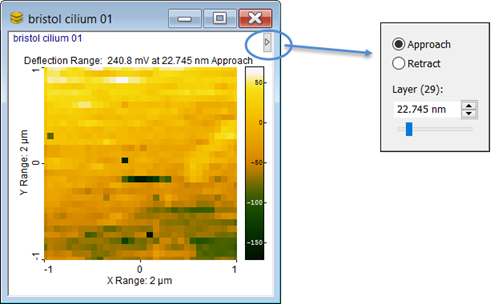
A volume image contains several layers and for the user it is possible to select the layer for which the belonging deflection signal should be shown.
This can be done directly from the image window or from a selected force curve:
By hoovering with the mouse over the arrow in the top right of the volume image a small dialog will appear and enable selection of the layer.
Alternatively the selection can be done by use of the marker tools in the force curve window as shown in the below figure.
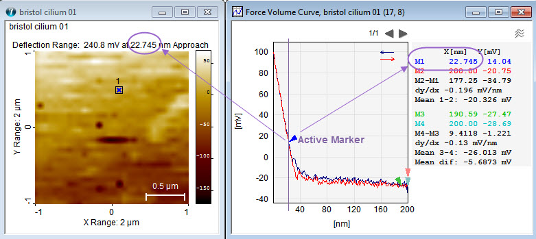
Image with courtesy of Dr. Terry McMaster, University of Bristol.
Another option is to combine the keyboard Shift key with the scroll wheel to select the height value for which the deflection values should be shown.
The displayed image is a map of deflection values at the height level (x-axis) of the currently Active marker in the Force Volume Curve window. I.e. the image is a cross section through all force curves at a chosen height level. There are two markers on the approach curve and two markers on the retract curve. When the active marker is on the approach curve the Force Volume image will be generated from deflection values of the approach curves. When the Active marker is on the retract curve the image is generated from the retract curves. Which curves are used is displayed inside the image window above the actual image together with the used height level.
Note that SPIP™ when an image has fewer pixels than the associated representation on the screen by default interpolates the screen pixels. This helps the eye to see shapes and other details in the image. Some other programs shows the image pixels non-interpolated, i.e. image pixels are displayed as squares. Interpolation can be switched on and off in the View Settings. The difference is illustrated below, where the left image is interpolated and the image to the right is displayed without interpolation.
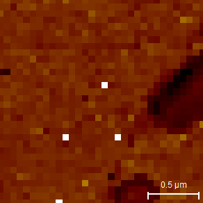
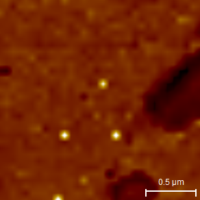
Image shown non-interpolated to the left and linear interpolated to the right.
Each individual displayed Force Volume curve is analyzed according to the current settings in the Force Curve Analysis Dialog. Results are reported in the graphs and in the reporting grid if chosen, but the data in the Force Volume Image remain unchanged. This means that Force Volume Curves can conveniently be analyzed and reported as if they were individual files.
Processing and analysis features working on the entire Force Volume image are available in the right click menu (or the Force Volume sub menu on the Processing main menu) on the Force Volume image.
For definitions and background please see the section on Force Curve Analysis elsewhere in this manual. The settings in the Force Curve Analysis dialog govern all processing and analysis of the Force Volume image.