
The Force Curve Analysis module enables you to perform advanced analysis of single force curve pairs, such as fitting models to pulling and indentations experiments and extract various parameters describing the physics. Furthermore, handling of Force Volume images are supported by interactive selection of individual curve pairs and mapping new images showing calculated forces, heights and extracted parameters for the individual curves. Therefore, it can provide new information on how adhesion and elasticity properties are distributed over the surface.
Force curves has their own contextual tab set in the ribbon called Force Curve Tools. This tab set will appear automatically whenever a force curve window is activated.

Some of the tools are generic and previously described for profiles. Here we will describe the functions, which are dedicated for force curves.

The View Panel differs from the generic view panel for charts, by having an additional "Show Dialog" button:
The Force Curve Analysis dialog will automatically appear when a new force curve window is created. This button can be used for defining another force curve as the curve to be analyzed in case more curve windows are present.

This function will perform a baseline correction using the settings defined by the force curve dialog in the Baseline tab
This function will perform a hysteresis correction of a force curve pair based on their height difference in their contact region (where the probe is in physical contact with the surface).
From the filtering pull down menu you can perform filtering by use of predefined filters or open the Filter dialog for interactive filtering.
The sign of the deflection signal can be inverted.

For averaging, comparing, or performing calculations on force curves it is an advantage to have the curves aligned in some way. Three alignment tools become active when a force curve window is switched into Comparison View.
Click this button in order to align all curves in the force volume image to start at at Height equal to zero.
Click this button to align all curves in the selected force curve window to have the same snap-in deflection value. If a single curve is selected, then all other curves will be aligned to this one. If no or several curves are selected then all curves will be aligned to curve number one.
Click this button to align all curves in the selected force curve window to have the same snap-in height value. If a single curve is selected, then all other curves will be aligned to this one. If no or several curves are selected then all curves will be aligned to curve number one.

Force curve pairs (approach and retraction) can be separated and shown in their own curve windows.
Click this button to calculate the average of all force curves in the selected force curve window and place the result in a new window. The average function will average the force curves as they are in the Comparison View, including any offsets made by dragging the curves around.
The force curve analysis dialog is activated either automatically when opening a file with force curve data or clicking Show Dialog tool key. When more force curve windows are present Force Curve Analysis focus is changed to the desired window by clicking the Show Dialog tool key, which will appear active when the selected force curve window is identical to the one being analyzed.
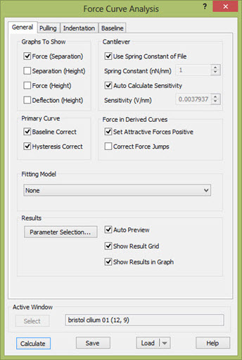
The Force Curve Analysis Dialog consists of four tabs, General, Pulling, Indentation, and Baseline.
The Baseline tab contains settings for baseline correction, the Indentation tab contains settings and user supplied parameters for the fitting of indentation models to the force curves, and the Pulling tab holds the settings and parameters for pulling experiments. The General tab contains buttons and check boxes for controlling the output, for choice of fitting model and toggles for correction and manipulation of the force curve data. In addition the General tab has fields for entering the cantilever sensitivity and the spring constant of the cantilever. Except for the toggles for data manipulation all relevant entered parameters and settings are shared with Force Volume image analysis.
The entered settings can be saved to Force Curve Settings (*.fcs) files and defined as default by saving the settings to the file called Default.fcs so that it can be loaded for another session.
To avoid accumulation of force curve windows it is often an advantage to enable the Close All Data Windows when Opening a File option (found on the File > Open Options) so that all data windows are closed whenever a new file is opened. You may also find it convenient to drag drop force curves from the ImageMet Explorer to the SPIP main frame.
In SPIPTM Force curves are assumed to be recorded with a cantilever-deflection sensor based AFM or similar apparatus. I.e. the bending of a cantilever spring is recorded as a function of the height of the fixed end of the cantilever. Hence, the data files are assumed to contain deflection (usually in voltage units) as a function of height, where height refers to the change in distance between non-flexible parts of the sample holder and the cantilever holder. Also the data files are assumed to contain both an approach and a retraction curve. By default SPIPTM displays approach curves in blue color and retract curves in red color and indicates the movement direction of the curves by red and blue arrows.
SPIP converts the cantilever deflection in units of voltage in to length units using the cantilever sensitivity factor. This factor is entered on the General tab in the Force Curve Analysis dialog in SPIPTM and is displayed in units Volt/nanometer. This factor can be measured as the slope in the contact region of the deflection vs. height curve recorded on a hard surface (e.g. a silicon surface); hard meaning with an elastic stiffness much higher that of the spring constant of the cantilever. Setting two cursors on one of the curves in the contact region of the deflection vs. height curve in SPIPTM will cause the slope dy/dx corresponding to the cantilever sensitivity to be calculated. SPIPTM can also calculate the sensitivity automatically based on the approach curve.
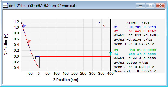
When analyzing and comparing multiple force curves from the same measurement series, the sensitivity factor should be determined once on a representative curve and the automatic detection should hereafter be disabled. When recording force curves of indentation type on soft surfaces it is a good idea to make a sensitivity calibration measurement on a hard surface at some point during the experiment.
In some cases the cantilever sensitivity factor has been determined prior to the acquisition of the force curves and the deflection in the data files has already been converted into units of lengths.
The cantilever deflection in length units is converted in to cantilever force by multiplying the deflection with spring constant of the cantilever which is also entered on the General tab in the Force Curve Analysis dialog in SPIPTM.
|
Deflection[nm] |
= Deflection[Volts] / Sensitivity |
|
Force |
= Spring constant ´ Deflection[nm] |
The spring constant may be measured by the use of a second calibrated cantilever or from the cantilever's thermal vibration spectrum, which the acquisition software of some AFMs can record. If the spring constant cannot be accurately determined the manufacturer's specification may be used, however with some caution. For some file formats SPIPTM can read the spring constant from the file if it has been entered during the measurement.
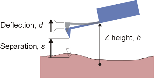
The separation (with the opposite sign of indentation) between the tip apex and the surface is given by the height change plus the change in deflection, both quantities counted positive up.
Separation = DZ-Height + DDeflection[nm]
When SPIPTM calculates the separation vs. height curves the origin is set at the point of deepest indentation. This may be counter intuitive from an indentation point of view where one would assume zero separation to be at the point where the tip contacts the undisturbed surface. Determining this point accurately is not trivial. Therefore there are several options available for the indentation fitting models.
Due to non-ideal recordings the force curves may need to be corrected. SPIPTM offers corrections methods for correcting baseline distortions and hysteresis described below. Furthermore, the force curves may be filtered by the filters available in the Filter Module where Gauss smoothing may be a good choice for removing high frequent noise.
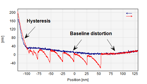
Force curve example showing hysteresis and baseline distortions
When the tip and the sample are separated by a large distance the cantilever deflection should ideally be zero. I.e. both the approach and the retract curve should be flat at large separations. However, often electrical offsets, drift, long range electrostatic forces and parasitic reflections in optical cantilever detection systems cause the curves to be non-flat and non-zero in these regions.
Baseline correction is toggled on and off on the General tab shown above whereas all settings are available on the Baseline tab in the Force Curve Analysis Dialog.
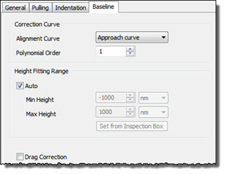
SPIPTM can correct the force curves by fitting a line of polynomial order 0 to 3 to either of the approach or the retract curve (Alignment curve) in the supposedly flat region of the recorded deflection vs. height curve. Thereafter the fit is subtracted from both of the approach and retract curves in the baseline region, which means that it will not affect the slope of the curves in the contact region. Thereafter the fit is subtracted from both the approach and retract curves in the fitting range and from data points to the right of the fitting range. Data points to the left of the fitting range are offset in deflection to joint seamlessly with the corrected points. Often when the tip comes in contact with the surface the long range forces and artifacts change their height dependence. Hence, it is not advisable to extrapolate the functionality from the non-contact region. This is why SPIPTM only corrects the contact region (supposedly left of the baseline fitting range) to zero order, i.e. by an offset value.
. Viscous drag on the cantilever may cause the approach and retraction curves to show different force levels even in the non-contact regime. This error can be corrected for by setting Drag Correction on. The drag correction is performed by adding a constant value to the curve Not given as the “Alignment Curve”. This constant value is found from mode value of the difference values between the approach and retraction curves in the defined baseline section. The drag correction will be performed for the entire curve.
The height fitting range used for baseline correction fitting can be set manually or SPIPTM can find an appropriate range automatically avoiding artifacts often seen at the far end of the curves. The height range can conveniently be defined by the inspection box in the force curve and clicking on Set From Inspection Box
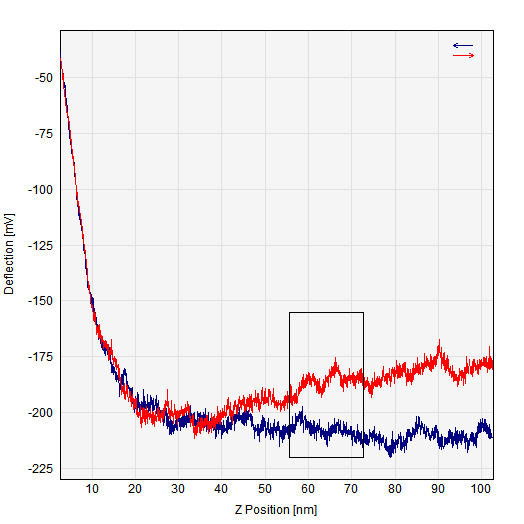
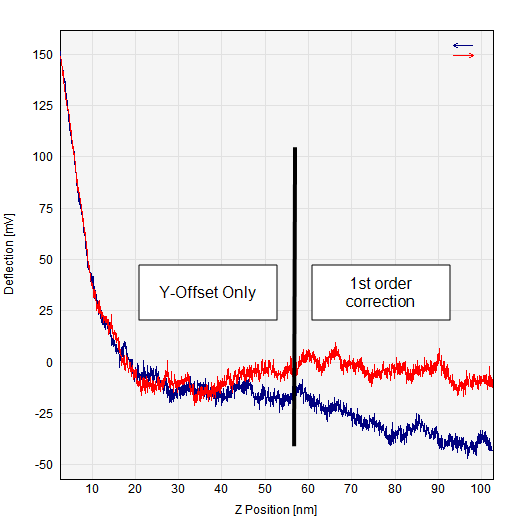
Baseline Correction Example: In the left curve pair the estimation area is defined by the inspection box, which was set to estimate the retraction curve. The right image shows the results after correction. The left part of the estimation area has only been offset by a constant value and the shapes of this part of the curves are therefore unchanged. On the right part the curves has been correction by a fitted line such that the retraction curve now is more horizontal.
Baseline correction is toggled on and off on the General tab whereas all settings are available on the Baseline tab in the Force Curve Analysis Dialog. Baseline correction can also be carried out on the active window by pressing the Baseline correction tool key ![]() .
.
Before performing any fitting to indentation or pulling models it is essential to baseline correct the force curves.
SPIPTM can to a large extend correct for hysteresis by shifting the retract curve so that it will overlap with the approach curve in the contact region. Due to hysteresis in the scanners used for moving then cantilever relative to the sample surface the approach and the retract curve is often not overlapping. Drift can also be the cause of this.
During a snap-in or pull-off event there is a high change in the deflection value and there may be too few sample points to express the force value correctly during the event. This may cause calculation of the dissipated energy to be less accurate. To compensate for this problem SPIP can modify the separation coordinates within the event range such that they equal the separation value of the local maximum adhesion point.
Below is seen how a force versus separation curve may be seen without and with Force Jump correction:
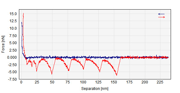
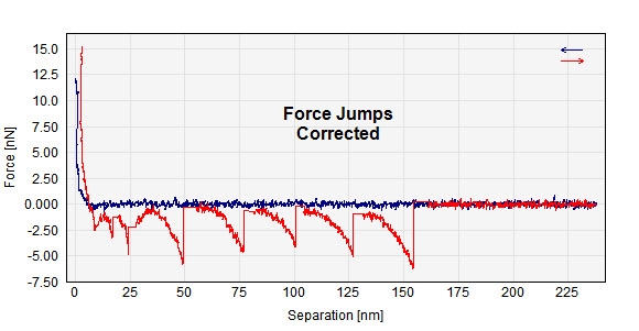
Calculated force vs Separation curves without and with Force Jumps Corrections
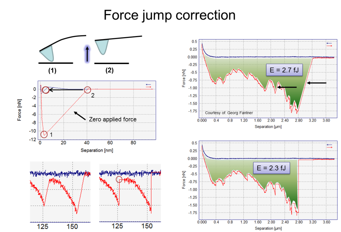
Most energy dissipation studies using force curves are about how molecules (adsorbed or part of the surface) are in-elastically stretched. Usually the stretching is terminated by a rupture event. After the rupture, there is no further energy exchange between the tip/cantilever and the molecule.
In order to calculate energy, it is not enough to know the piezo position (the horizontal axis on the raw force curve). We actually need to know the molecule extension (equal to tip -surface separation), because the way energy is calculated is by integrating the force as a function of the tip-surface separation.
We calculate the tip-surface separation (molecule extension) by adding the piezo position and the cantilever deflection.
What happens at the rupture is that what appear as a vertical force jump in the raw force curve is converted to an oblique line in the force-separation curve (see the slides I sent you). When integration the force for the energy calculation one should really stop in the left end of this transition. Otherwise, the energy will be overestimated.
In order to avoid making decisions behind the scenes about starting/stopping integration we have chosen instead to modify the curve wherever a rupture event is detected. This way the user can see what is happening. This makes the software more robust and clear to understand, in particular when analyzing curves with multiple ruptures.
The energy is calculated as the area between the approach and the retract curve.
The approach curve is also force jump corrected which means that a snap in, if present, is also corrected. Usually the snap in is caused by conservative forces (electrostatic, vdw, magnetic) resulting in no net energy exchange. So again, for most practical "energy" experiments we don't want the influence of snap-in.
Sometimes it may be convenient to show the attractive forces as positive and the repulsive forces as negative forces, e.g. when analyzing curves from unfolding protein experiments. This can be set by the Set Attractive Forces Positive check box.
Using the principles described above SPIPTM can generate the Force vs. Separation plot, Force vs. Height plot, the Separation vs. Height plot and the Deflection[nm] vs Height plot. Usually the Force vs. Separation plot will be the most interesting, since it is on this plot all fitting and event detection takes place.
It is possible to choose between two indentation models and one pulling model which will be fitted to the Force vs. Separation curve. The indentation models are the Hertz and Sneddon models for the indentation of a rigid sphere and a rigid cone, respectively, on a soft flat surface. For pulling experiments the Worm Like Chain (WLC) model is available. When the WLC model is chosen, the peak force and the unloading rate are reported for all detected unfolding/rupture events. For details see the corresponding sections below.
A list of the available numerical results belonging to the various fitting models and event detections can be found at the end of this chapter. The results are captured to the table – or grid - in the Force Curve Analysis Results window and/or directly in the shown graphs. The display of the calculated numerical results can be toggled on and off with the Show Results Grid and the Show Results in Graph check boxes.
In the Results section you can define which parameters you want to calculate and how to show them.

To chose between the available parameters to be calculated click the "Parameter Selection" button which will open the Force Parameter Options dialog:
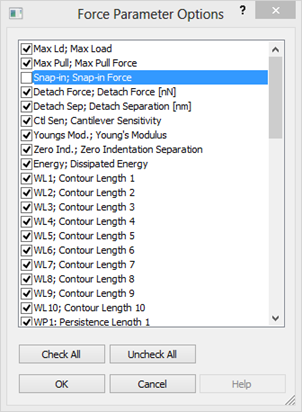
See more details in the Force Curve Parameters section.
When auto preview is set the desired output curves will be calculated together with selected force curve result parameters, when browsing through force curves already included in the force curve window or when adding selecting new force curves, for example from a force volume image. However, the results will not be stored to the result grid before the Calculate button is pressed.
Use this check box to turn the Force Curve Result grid On/Off..
In addition to having the numerical results shown in the result grid it is possible also to have the values to appear in the Force versus Separation window.
When clicking the Calculate button the desired parameters and derived curves will be calculated and the numerical results will be put into the Force Curve Results window. If the source window is shown in Analysis View (only one curve show) only the shown curve will be analyzed. In contrast all curves contained in the window will be analyzed when the source window is in Comparison View mode.
SPIPTM has two models implemented, which can be used to derive the Young's modulus (the elastic modulus) from indentation curves. In both models it is assumed that the modulus of the tip is much higher than the modulus of the surface. The models can be fitted to either the approach curve, theretract curve or the calculated average curve. The Fitting model is defined in the General tabwhereas the settings for fitting the indentation models are defined in the Indentation tab
Sphere Indentation (Hertz). In this model [Johnson et al.] a rigid sphere is indenting a flat soft surface. No adhesion and no visco-elasticity are assumed. The model is only valid for indents, which are small compared to the radius of curvature of the tip. Therefore, to make use of this model, sharp AFM tips cannot be used for the experiments. Instead rounded tips or spheres attached to a cantilever should be used for indentations of more than a couple of nanometers.
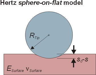

|
ESurface |
Young's modulus for the surface |
|
nsurface |
Surface Poisson's ratio. 0.5 for perfect rubber 0.31-0.35 for most metals |
|
Rtip |
Ball radius of the tip in the Hertz model |
|
s0 |
Point of zero indentation, i.e. the level of the undisturbed surface |
|
s0-s |
Indentation. Note, that S is counted positive upwards.
|
|
Assumptions: |
ESurface << ETip, S0-S << Rtip, no adhesion, no visco-elasticity |
This model [Derjagin, Muller, Toropov, 1975] is similar to the Hertz model and takes the long range attractive forces into account by substituting the point of zero indentation with the point of max adhesion.

|
sm FpullOff |
Max adhesion distance Pull off force |
The Johnson-Kendal-Roberts (JKR) model is an extension of the Hertz model taking into account short range adhesive forces caused by minimization of surface energy. It differs from both the Hertz and the DMT models in the fact that the soft surface will stick to the tip (sphere) during the retract process and form a neck, which will shrink and at some point break. The model is applied to the retract curve only and is valid only when the surface is much softer than the tip (assumption Esurface << Etip).
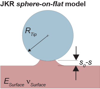
Contact radius:

Surface reduced modulus (see definitions for the Hertz model):

Surface energy (work of adhesion):

The work of adhesion can be calculated from the maximum adhesion force. By identifying the point of maximum adhesion and the point of zero separation (zero indentation) it is possible to calculate the reduced modulus as proposed by Sun et al [49], see also [50,51].
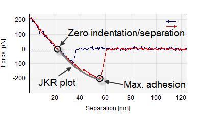
The JKR equation is plotted between the zero separation point and the maximum adhesion point using the following approximation for the relation between contact radius and surface deformation Capella et al [48]. The assumption is that the contact radius is much smaller that the tip radius. Note that the displayed curve this is not a fit, but deduced from the Zero indentation and Max. adhesion points!

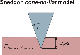
In this model [Sneddon, Radmacher, Domke et al.] a rigid cone is punched into a soft flat surface. Again, adhesion and visco-elasticity is assumed to be absent. As AFM tips may be conical but not infinitely sharp the model woks only when the indent is significantly higher than the radius of curvature of the tip apex.

|
a |
Tip half cone opening angle |
|
Assumptions: |
ESurface << ETip, s0-s >> Rtip, no adhesion, no visco-elasticity. |
You can control various parameters for detection of indentation points and calculation of the Young's Modulus from the Indentation tab of the Force Curve dialog:
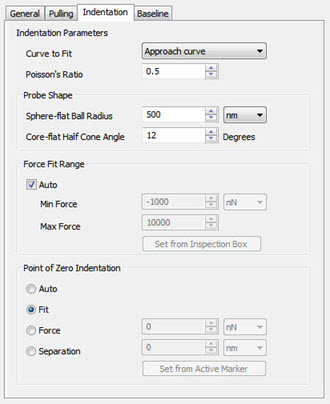
The user has to provide parameters to the fitting routine such as the geometry of the tip and the Poission's ratio of the surface material and optionally the point of zero indentation, s0, and the force range used for fitting.
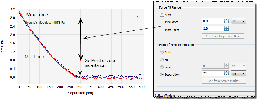
The Point of Zero Indentation/separation, s0can be chosen manually at either a fixed force level or a fixed separation and refers to the Force vs. Separation curve window. The value can be entered directly in the Indentation tab or transferred from the position of the active cursor in the force vs separation plot by pushing the Set from Active Markerbutton in the Indentation tab.
The choice of s0 is crucial for the quality of the fitting. Therefore SPIPTM additionally provides the possibility for finding this point automatically or finding this point as a result of the fitting procedure. When SPIPTM finds s0 automatically (Auto) the force vs. separation curve is searched from left to right to the point where the force becomes equal to or less than the baseline level.
Also the force range used for the fitting can be chosen explicitly or chosen automatically by SPIPTM. A range can be manually chosen using the inspection box and thereafter pushing the “Set from inspection box” button in the dialog. In Auto mode the minimum force level is set to the force level at s0 and the maximum force level is set to the maximum indentation force taking leaving out a possible saturated region.
When the Worm Like Chain (WLC) model is checked a WLC [Janshoff et al.] model will automatically be fitted to each detected unfolding event. The model is based on the following formula:

Where FWLC(s) describes the Force as function of separation s, kB is the Boltzmann's constant, T the temperature in Kelvin, lpthe persistence length and Lc the contour length, which are reported as the results and optionally presented in the graph. In addition the peak force and the separation and un-loading rate at rupture are reported.
When more than two unfolding events are detected the individual Contour Length results will be displayed as function of the event index. The slope of this graph is automatically calculated and reflects the domain contour length in the protein.
Settings for the detection of pull off events and model parameters can be entered in the Pulling tab:
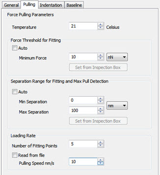
Temperature (in degrees Celsius) is the only constant which the user has to supply.
The Separation Rangeused for detection of the pull off events can be automatically chosen by SPIPTM or the user can type in a range. The range can be selected interactively using the inspection box on the Force vs. Separation plot followed by a click on the Set from inspection Box button.
Force Threshold. In order to restrict detection of unfolding events to high forces a threshold can be typed in. The threshold can be chosen interactively using the inspection box on the force vs. separation plot followed by a click on the Set from inspection Box button.
The Number of Fitting Points used for calculating the pulling speed at rupture (the unloading rate) can be adjusted and should be chosen large enough to suppress noise and low enough to get a reliable estimate. The actual choice depends on the sampling density in the recorded curve.
Pulling Speed. For some file formats SPIPTM can read the scan rate corresponding to a pulling speed from the data file. In other cases it has to be entered in order to get the correct scaling of the reported un-loading rates.
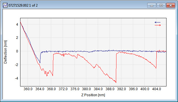
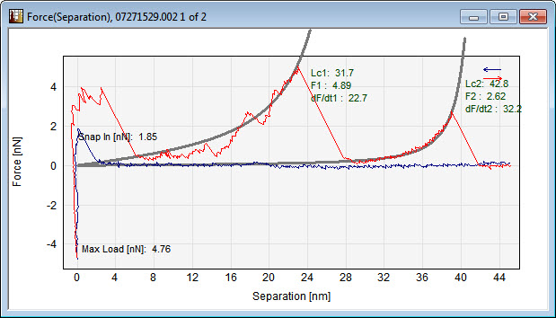
Worm Like Chain Model analysis example. To the left is the recorded Deflection vs. Height curve. To the right the calculated force vs. separation graph is shown with two fitted WLC models. Also the rupture force and the unloading rate for the first unfolding event are displayed.
Data Courtesy of Michael Wrang Mortensen, Danish Institute of Fundamental Metrology.
Numerical results are captured to a grid (or table) in the Force Curve Results window. When results are captured to the Force Curve Results grid only one entry per file is allowed. This means that when e.g. fitting parameters are calculated only the last calculated result will appear in the grid. It is possible to delete single rows or all rows of the grid through the right click menu where which is also used for copying the contents to the clip-board.
A brief description of each parameter that can be selected for calculation in the Parameter Selection window is given below:
Max Pull Force is the maximum pulling force on the retraction curve. Often this will be identical to the detachment force (Detach Force).
Snap-in Force is the magnitude of the force immediately after snap in.
Max Load Force is the maximum loading force usually at the left end of the approach curve.
Detach Force is the force before the last event on the retraction curve, corresponding to the point where the tip and the surface loose contact.
Detach Separation is the separation (distance between tip apex and the maximum indentation point) at detachment.
Young's Modulus is the elastic modulus calculated by one of the indentation fitting models on the Force vs. Separation curve.
Cantilever Sensitivity is the sensitivity factor used for the calculation of the parameters. It is reported since it can be automatically calculated (from the approach curve) and hence different for each force curve.
Zero Indentation Separation is the point in the Force vs. Separation graph which is used as zero point for indentation fitting.
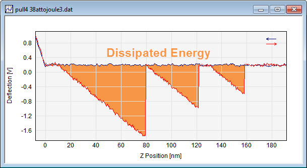
Dissipated Energy is calculated as the area between the approach curve and the retraction curve of the Force vs. Separation curve, see picture below. At sites where the retraction force exceeds the approach curve the in between area is regarded as negative.
WL1..10 are the contour lengths resulting from Worm Like Chain model fits to each detected unfolding event.
WP1..10 are the persistence lengths resulting from Worm Like Chain model fits to each detected unfolding event
WF1..10 are detected peak forces for each detected unfolding event when the Worm Like Chain Model is applied.
DF1..10 are detected unloading force rates for each detected unfolding event when the Worm Like Chain Model is applied.
WS1..10 are the separation values for each pull off event when the Worm Like Chain Model is applied.
A batch process including Force Curve Analysis will automatically generate an ASCII file with a table corresponding to the result grid. Likewise optional reports in HTML and MS Word can be generated. For high throughput it might be desirable not to include the HTML and MS Word reports, to save processing time.
To perform a simple batch process for a large number of files you should open the Batch Dialog and include the "Force Curve Analysis" among the available functions. Then you may select a group of files / folders containing force curve files and drag-drop them into the SPIP workspace. The Batch Process will use the most recent Force Curve Analysis dialog settings or the settings saved under the name Default.fcs if it exists.