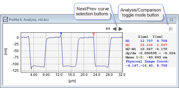
Cross section profiling is performed by marking one or more cross-section lines in an image window by use of one of the profiling tools found in the General Ribbon > Cross Section Profile Group .

The Analysis view enables you to perform interactive measurements on a selected curve by the cursors and it also has a number of automated functions such as histogram analysis. In contrast, the comparison view allows you to compare all marked profiles but the analytical functions are very restricted.
The left/right arrow buttons at the top of the window enables you to browse through all marked profiles.
The number of cursors can defined in the Profile View Settings and their functions related functions are described in the Profile Cursor Functions section.
In some situations you may have a profile disconnected from an image, and in such case it will be shown in a window denoted "Single Curve Window". It will have most of the same analytical tools except those related to the source image and the Comparison View mode.
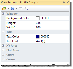
From the Cross-section View Settings the appearance of the profile window can be controlled.

Most of the settings are self-explained so here we will primarily introduce the more advanced settings.
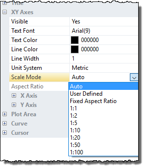
Initially the Scale Mode is set to Auto, which guarantees a graph covering all data with optimal use of the window space. In case you want to study the curves at a certain scale you can define the X, Y Axis individually by choosing the "User Defined" Scale Mode.

For topographic profiles you may set a "Fixed Aspect Ratio" such that the y values are scaled by the given factor compared to the x-axis. You may also choose between one of the predefined x:y scaling. The one of most interest might be the 1:1 aspect ratio because it will show the profile in the correct geometrical scale, such that angles seen on the screen output will be identical to the physical angles.