Plane correction is one of the most important aspects of SPM image correction. SPM instruments often have a non-linear coupling between the lateral plane and the Z-axis causing unwanted bow in the image. The process for plane correcting the surface image is also called "flattening". Image flattening can be a challenging process, especially when the surface structure contains steps most flattening algorithms will fail because they cannot distinguish the real structure from the plane distortions. However, SPIP has dedicated tools for detecting and handling steps such that the individual steps will appear flat.
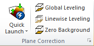
The plane correction can be performed directly from the Ribbon using the General > Modify panel or the Modify > Plane Correction Panel:
The Global and Linewise Leveling serves as quick access to 1st order plane correction methods that will work relatively well for most images. The Zero Background tool will set the background z-value to zero where the background value is defined as the most frequent z-value found by histogram analysis.
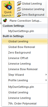
Clicking on the Quick Launch button will provide direct access to Built-in and Custom settings, which will be applied when selected:
The Plane Correction dialog can be opened by clicking on Plane Correction Setup... or the Dialog Launcher  ,
,
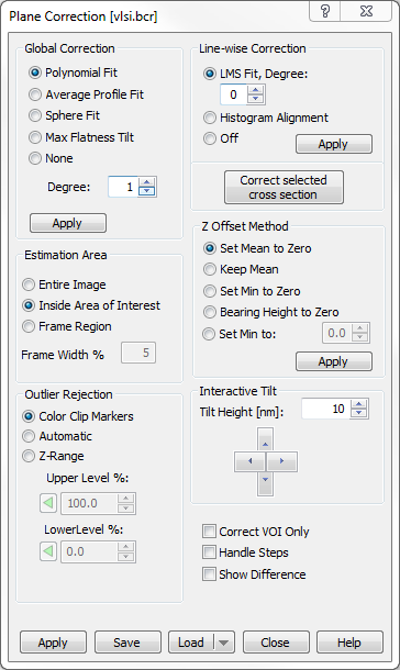
It is possible to select between four different plane correction algorithms that subtract a fitted image to the global image:
Polynomial Fit, Average Profile Fit, Sphere Fit and Max Flatness Tilt.
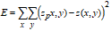
Slope corrects the image based on a Least Mean Square fit to the entire image or the volume defined by the Estimation Area group box. To the image z(x,y) a plane zp(x,y) is fitted by a polynomial function of the form:

The coefficient ai and bi for the polynomial function is then found by minimizing the Square Sum Error:
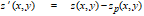
The corrected image z'(x,y) is then calculated by subtracting the fitted plane:
The computation time for estimating the plane parameters can for some applications be inconvenient especially for images containing a large number of pixels. In those cases the number of operations can be reduced by letting the plane fit be based on the average x and y profiles. An average x profile is found by adding all individual x profiles into a single curve and the average y profile is found similarly:


From the x and y profiles the two sets of, a and b, coefficients is determined within a very short computation time.
Polynomial degrees for the two Least Mean Square fit methods can be set between 0 and 5. Degrees greater than 3 are seldom recommended because the fit might then start to match the real surface structure more than the undesired plane error.
This will subtract an estimated sphere form.
Enabling Max Flatness Tilt will automatically tilt the image so that the height distribution histogram will maximize the frequency a dominating height level. When SPIP detects two dominating height levels, it will maximize the sum of those two frequencies. This function has it advantage when dealing with single steps where the polynomial fit functions may fail because they will fit functions to the step rather than undesired image bow.
When setting the Global Correction method to None, no automated Global correction methods will be performed even when "Apply When Loading" is checked.
Press the Apply button in the Global Correction group box to apply the global correction method.
Small surface corrugations can sometimes be dominated by the noise in the scanner system. Typically, this creates observable steps between subsequent scan lines. Likewise, temporary contamination of the probe will cause the scan lines to be leveled differently.
In such cases the image can be corrected by leveling the individual scan lines to more probable levels. SPIP offers two methods that can be combined with the polynomial plane correction.
The LMS Fit method subtracts a fitted polynomial function from each individual scan line with at polynomial degree defined by the Degree numerical text field.
The improvement may be astonishing. However, there might be less information about corrugations perpendicular to the scan lines. Especially for roughness measurements, this may cause underestimated values.
To achieve the best results it will often be an advantage to combine this method with the Inside Color Range check box of the Estimation Volume set. When doing so it is possible to eliminate the influence of noise, particles and real surface corrugation and concentrate on the bow artifacts created by the scanner.
This correction technique elevates the individual x-profiles so that their height distribution obtains the best match. The result will be reflected immediately in the height distribution histogram for the image, which will show the dominating height values as sharper peaks.
For structures where the average value of the profiles may vary, for example, waffle patterns for height calibration references this technique is particularly valuable.
The method is especially powerful in connection with Z-calibration.
The line-wise settings can be applied independently from the other settings using the dedicated Apply button.
This function is ideal for interactive elimination of local scan line distortions.
To correct a single scan line or horizontal line piece, create at horizontal cross-section and press the "Correct Selected Cross-section" button. You can also limit the part of the cross-section, which you want to correct by applying cursors in the profile window. When the cursors are shown only the line piece between the cursors will be corrected.
The correction will substitute the pixels on the cross-section line by the average value of their upper and lower neighboring pixels.
To correct more scan lines simultaneously you can apply Average Profiling . The averaging box will define the scan lines to be corrected, the new pixel values will then be found by interpolation.
The same method can be performed by right clicking in a profile window on Cursor Function > Correct data between cursors by neighboring scan lines
The fitting of the plane used the plane correction can be restricted to specific parts of the image area, so that only in-plane parts are used. This can be done using Area of Interest Markers or by specifying a band along the image border inside which the fitting takes place.
The slope correction will be based on the entire image area.
The estimation of the plane used for correcting the image can be limited by Area of Interest Markers (AOI). Specific regions can be included, for example a single terrace on a stepped surface, or two narrow bands in each side of the image for line wise leveling - or just three small areas for three-point (3-point) leveling. However, often it is the inverse AOI markers which are used in order to mask out (block) areas in the image containing coarse structures.
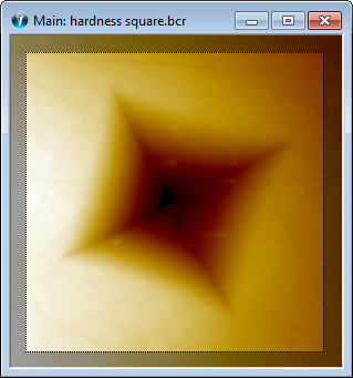
The plane fit will be based on a narrow band along the image border. This is particularly useful when the center part of the image contains a dominating feature like, for example, an indentation that could cause wrong estimation of the surface bearing plane. As the estimation area often becomes quite small it is advisable to use this option only with first order fitting. Further, as the top and bottom lines in the image are not masked at all, it is not advisable to use any line wise correction with the Frame Region option.
The estimation of the fitting plane is taking place inside a narrow band along the image border, here shaded in black.
The frame width can be set between 1 and 30% of the image width.
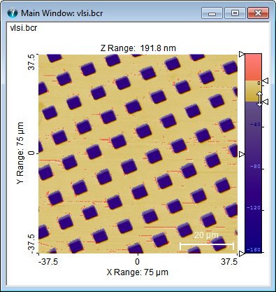
When this setting is set the estimation area is (further) limited to the pixels having Z values within the upper and lower color clip limits of the color scale. This enables a plane correction without influence from outliers or asymmetric distributions of for example particles, pits or terrace. Below is seen how the color scale clip markers are used to define the Z-range, which will be used in the estimation of the plane structure; the blue and red areas will be ignored.
Often it is necessary to perform plane correction iteratively using Z range restriction to achieve optimal results.
SPIP™ can automatically find outliers and mask them out when performing the plane fitting, this saving the user for two iterations of Plane Correction with color clip marker adjustments. The Auto function is particularly useful in connection with Batch Processing, where the user has no possibility for adjusting color clip markers. Three built-in settings using automatic outlier rejection for use with QuickLaunch are installed with SPIP™.
In particular, for use with Batch Processing it is possible to save Plane Correction settings with a specific Z-range (color clip marker range) defined. The range is defined in percent of the full Z range of the active image, so that a saved setting can be used easily with images having different Z ranges and Z offsets. In a Batch script will often be advantageous to first apply a Global Leveling of the image before applying a Plane Correction setting with restricted Z Range.
As this option can be combined with the Estimation Area options described above it is possible to determine an estimation volume rather than just an estimation area or z-range.
It is highly recommended to use this option for accurate step height measurements.
Only the pixels inside the Area of Interest and pixels having values within the range defined by the Color Scale markers will be corrected. The surrounding will be leveled by constant values so that no or only small edges will appear.
This setting is especially useful when correcting images containing steps and where the nature of the distortion on the individual steps is different. In such case you should use the color scale markers and the AOI tools to define and correct one step at a time.
The Plane Correction Dialog offers five ways of setting the Z Offset:
This will level the image so that the mean value of the image is set to zero.
This will level the image so that the mean value of the original image is preserved after a plane correction.
This will level the image so that the min value of the image is set to zero.
This will define the bearing height as the most dominant height value (based on a height distribution histogram) and level the image so that it is set to zero. The dominant height value is identical to the value in the height distribution histogram having the highest frequency. The number of bins used in the histogram is the minimum of 1000 and the number of points in the images, - so in most cases it will be 1000.
You can also level image such that the minimum value is set at a specific value by checking the associated radio button and entering the desired min value.
The selected Z-Offset method can be applied independently from the other settings by clicking on the Apply button in the Z-Offset Method group box.
The plane of the image can be tilted manually by use of the arrows and the tilt step can be controlled by the Tilt Height number entered in nm. It is possible to monitor the effect on the histogram distribution and a profile simultaneously by having these windows open.
For images containing significant steps it is recommend setting the “Handle Steps” option on. In such case SPIP will combine a number of algorithms to detect and handle steps such that the flatness is optimized. This option is always applied when using the “Quality Priority” mode. A detailed description of the algorithms is a company secret and cannot be revealed. If it is important for you to document the algorithm used you should not use this option.
When this option is on the difference between the image before and after correction image is shown. This image is identical to the correction image and describes exactly how the image was corrected in the most recent correction.
You can save the actual settings into file such that they can be recalled again. When saving into the file called “Default.pln” you will define the default settings which will be loaded when restarting SPIP. Stored settings files can also be recalled from batch processes so that results from batch processes are independent from actual user modified settings.
When clicking on the Apply button at the bottom of the dialog the selected slope correction methods will be applied on the Main Image. The result is immediately reflected in the profile curve and the histogram if open.
If you are using the Custom mode, it can sometimes be necessary to process the image more times with different settings. In such case, it is an advantage to monitor the histogram and a representative profile while adjusting the image plane. They are updated simultaneously with the image and you can easily see if the image is improving.
To avoid the influence from outliers, such as spikes, particles, pores and indentations you should apply the Inside Color Range option and the color scale markers in the image window to define a valid z-range for the estimation volume, such that the outliers will have little or no effect on the result. Likewise, you may apply the Inside Area of Interest option combined with the AOI tools to exclude outlier areas.
If you are having specific outliers in the image which you want to reduce you can use the outlier objects filter of the filter module or the following trick:
Mark the outlier area by AOI tools such that the exterior is defined as the Area of Interest.
Select the AOI Frame, right click on it and click “Define Outside AOI's as Void Pixels”
Right click in the image on “Void PixelsàInterpolate new values”
Right click in the image on “Void PixelsàAccept
While working with plane correction undesired results may occur, in which case you can take advantage of the undo function just by clicking Ctrl+Z. To learn more about the undo function, see the Undo section.