The Outlier Objects Filter is a strong tool for detecting outliers and filling in the most probable values by interpolation of neighboring pixels, where the aim is to get the truest representation of the image. SPIP will detect a particle when some part of it exceeds a certain level and will then determine its boundaries at the positions where the slope of the particle flattens or changes sign. A user-selected Exchange Method will then fill the pixels inside the particle boundary. Instead of particles it is also possible to detect and remove spikes exceeding a certain slope threshold.
The Outlier Objects Filter is activated by clicking Modify > Filtering > Remove Outliers of the Image Tools in the ribbon.
The upper part of the dialog define which features should be removed, Particles, Pores, Spikes or NegativeSpikes.
The Detection Level is set as a percentage of the z-range of the image. Because the Z-range of the image will decrease for each filter process, it is possible to filter the image gradually by setting a high detection level and pushing the Apply bottom more times.
The detection level will be reflected on the color scale so that you see which part of the images will be handled as objects to be filtered. Likewise you can also define the color scale of the image or the color scale editor. For particles the upper color scale limit will define the threshold value and for pores the lower color scale limit is associated with the threshold value.
When the "Spike Exceeding Slope" is checked the slope level for detecting a spike can be set. A spike is defined here as a local maximum, or minimum for negative spikes, where the slope dz/dx or dz/dy exceeds the set slope level. Here, we regard maximum values as pixels which two neighboring values in X, or the two neighboring values in Y are smaller and vice versa for minimum values. Thereby it is possible to remove structures, which look like ridges, see example below.
Notice that for scanning probe images the maximum measurable slope is limited by the shape of the tip. If spikes have slopes larger than at the tip apex we have a good indication of a noise artifact, which should be filtered. This spike filter is therefore also very good for preprocessing images before tip characterization, which success depends on how well local maximums can be trusted.
The slope of the scanning tip may be different seen from different directions and it might also have been mounted so that for example, the tip is able of scanning side walls in one direction. In such situations, high slopes in one direction may be acceptable but not in the others and therefore necessary to handle the directions individually. To do this you can with the direction check boxes (Up, Down, Left and Right) define which slopes the spike detection algorithm will check against the given slope threshold value.
There six methods for filling new values into the "bad" pixels:
Horizontal Interpolation, where new values are inserted by interpolation of the neighboring values in the x-direction. This method is recommended for structures mainly oriented in the x-direction.
Vertical Interpolation, where new values are inserted by interpolation of the neighboring values in the y-direction. This method is recommended for structures mainly oriented in the y-direction
Min value, where a fixed value equal to the minimum value of the image is entered.
Mean Value, where a fixed value equal to the mean value of the image is entered
Median Value, where a fixed value equal to the median value of the image is entered
Fixed Value, where a value defined by the user is entered
Mark as Void, the outlier pixels will be marked as void pixels.
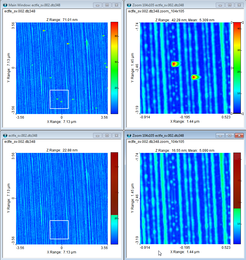
Below is seen an example of an AFM image with a fiber structure suffering from some contamination particles before and after filtration. At the top is the raw image together with an Inspection image focusing on two contamination particles and below is seen the same areas after filtration.
In this case the vertical interpolation method has been applied because the fiber direction is roughly parallel to the y-axis. It is seen that particles have been removed with very little or non-damage to the fibers and we will be able to quantify the fibers much better by Particle and Pore Analysis.
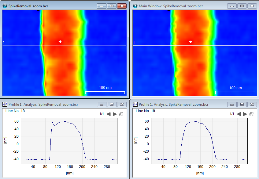
The next image demonstrates the effect of the Spike filter. The raw image at the top suffers from overshoots on the left wall, which is probably due to a change of probe angle, when the probe moves from low high friction to low friction. Such a spike may cause a tip characterization to overestimate the sharpness of the tip and it should therefore be eliminated before the tip characterization takes place.
In this case the spikes have been exchanged by horizontal interpolated values, and the result shows successful spike elimination with no damage to the remaining image.