The SPIP tip characterization module allows you to characterize the tip or stylus used for scanning the actual image. The basic methods used are very similar to the blind reconstruction method described by J. S. Villarrubia and P. M. Williams et. al.
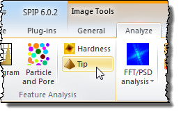
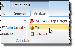
![]() The tip characterization can run on topographic images and profiles. For images the Tip tool key is located in the Feature Analysis panel of the Analyze tab. For profiles the tool key is located in the Calculate panel of the Analyze tab group:
The tip characterization can run on topographic images and profiles. For images the Tip tool key is located in the Feature Analysis panel of the Analyze tab. For profiles the tool key is located in the Calculate panel of the Analyze tab group:
If you have the Batch Processing option included in the software you can also run the tip characterization and Deconvolution in a batch process and combine it with other functions and thereby improve your productivity. There is four tip processing functions available for batch processing: Tip Deconvolute, Tip Characterize, Tip Load and Report Tip Characterization to HTML.
Likewise, it is possible to combine the Correlation Averaging on repeatable structures and thereby minimize the influence from noise.
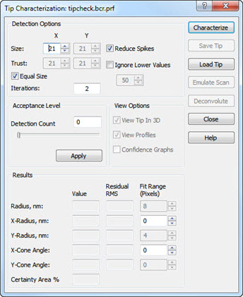
In the Tip Characterization dialog different detection parameters influencing the result can be set. It is important to notice that if we can assume that there are no image distortions, apart from tip artifacts; SPIP will be able to calculate the worst case tip. The worst-case found tip is able to scan all parts of the surface with its apex but might be sharper in reality.
The Size parameters defines the number of pixels for the tip to be estimated, uneven numbers in the range 3 to 255 are possible values for the X-dimension while the Y-Dimension can be set between 1 and 255; Having uneven pixels means that the tip apex always will be centered.
The X, Y tip length cannot exceed half of the respective surface image length. By setting the Y-length to 1 pixel it is possible to calculate the x-profile of the tip rather than a tip image. This is useful for 1 dimensional surface structures where tip information only can be obtained from one direction.
The Iteration number determines how many times the recursive algorithm will run through the image. First time the tip is evaluated only from the true maximums. Based on this tip we can create the Certainty Map by emulating a tip scan. This image tells us which part of the image that is scanned by the apex and can be trusted. In the second iteration all local maximums in the trusted image areas are used for further tip estimation and a new Certainty Map is created. Third and higher numbers of iterations are similar to the 2nd but now all trusted pixels are included. The computing time depends linearly with the number of iterations and it will seldom be necessary to use more than 3 iterations.
Trust pixel area defines how many pixels are trusted in 2nd and following iterations.
When estimating a large area of a tip the uncertainty of the border points will be much lower that the center pixels and can reduce the Certainty surface area because it will be difficult for the tip to enter the lower surface levels. This means that there will be fewer places where tip shape information can be deduced resulting in a too blond tip. If this is a problem it can be an advantage to define the Trust pixel area to be smaller than the tip area meaning that we are ignoring the tip outer parts when calculating the certainty area.
In most cases you should keep the Trust area equal to the tip size but especially when performing the characterization on pores rather than particles this option can be useful.
Depending on the image quality the tip characterization result may be influenced by noise and this is especially true when there are noise peaks creating maximums that are going to be used by the first iterations of the characterization algorithm. In these cases it is therefore important to have an intelligent way to reduce noise peaks. When the Reduce Spikes option is set, the tip is pre-calculated using only the first iteration described above. From the x and y profile of the tip the slopes at the very apex are evaluated. If the slopes at the very apex is higher than the slopes just below this is regarded as a noise artifact. In this case the height at the tip apex is then lowered so that the slopes at the apex does not exceed the slopes just below. Using the knowledge of the noise reduced tip we are now able to detect all parts of the image where we have peaks sharper than the tip and then reduce these values so that they in the following iterations doesn't causes the sharpness of the tip to be overestimated.
Note that the input image will be changed by this procedure, but you can regard the technique as an intelligent way of detecting and removing noisy peaks.
By checking this check box it is possible to ignore peaks in the lower parts of an image. This will shorten the processing time and limit the unwanted influence from small noise peaks. It is especially useful when applying dedicated tip-characterizing samples where the vital information is found in the upper part of the structure.
The level can be defined by the right color scale markers or the associated arrow keys.
If there is noise in the image, especially spikes, the sharpness of the tip can easily be overestimated. In such cases it is a good idea to increase the tip detection count, which is the number of occurrences in the image that a certain part of the tip would be inside the surface. This can of course not be true but is a way of ignoring the spikiest parts of the image. After the tip has been characterized you can set the detection count interactively by the scroll bar and in real-time observe how it changes the estimated tip. Note that the Acceptance level will influence the Certainty Map and thereby alter the tip estimation after 1st iteration in the tip estimation algorithm.
When pressing the Characterize button the tip characterization will be started and it will be based on the image window for which the tip characterization was invoked the first time.
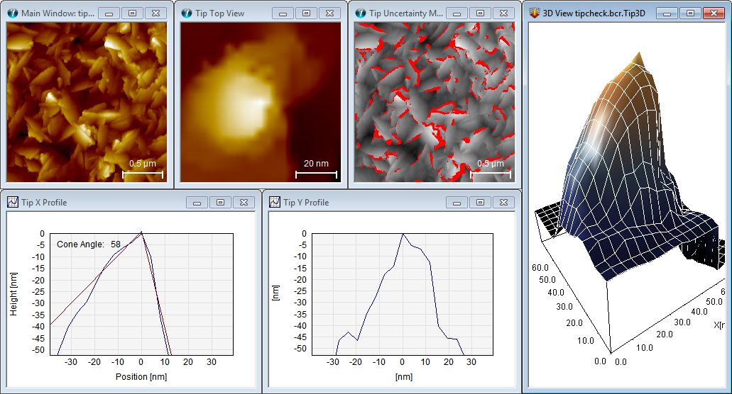
Below is seen a screen dump after a tip characterization with the estimated tip seen in top view and 3D perspective. The gray image is the Certainty Map and is the result of a tip scan emulation by the estimated tip and the surface image. The red marks indicate the positions where the tip is probing the surface with other parts than its apex.
Also the tip x- and y-profiles can be shown with their estimated tip radius (based on a circle fit) and the cone angles.
The following image is an AFM image of a dedicated Tip Characterization sample and demonstrates a blind reconstruction of the AFM tip.
After having estimated a tip you can save it in the BCR format, load it again and use it for Deconvolution of other images.
If the resolution (physical distance between pixels) of the loaded tip is different from the image to be de-convoluted the tip will be resampled to obtain the same resolution and a message will be given.
By the Emulate Scan push button it is possible to scan the Main Image with the current tip shown in the Tip Top View window, this process is also called dilation. The resulting image is called the Certainty Map because areas un-touched by the tip apex are detected and marked with the red color.
It is possible to use this function on artificial tips and surfaces and learn how different tips can affect the observed images and the quantitative results.
Deconvolution is important for correct line width measurements and can also assure more accurate results in particle size analysis and roughness measurements.
Pressing the Deconvolute button will calculate a new image based on the source Image and the actual tip shown in the Tip Top View window, this technique is also known as erosion. The process has only meaning when the surface structure has sharper edges than the tip. In such cases it is partly possible to correct for the width of the tip, which otherwise causes line width and the lateral size of particles to be overestimated.
A number of quantitative results can be extracted from a tip characterization process, which can be reported into Word files or HTML files when using batch processing and/or the Active Reporter
The Tip Radius is determined by a sphere fit to the estimated tip. Small radii characterize quality tips. The Radius is calculated from a sphere fit to the NxN center pixels where N is specified by the Fit Range input field. You can turn off the calculation by setting the Fit Range to zero.
The Tip X- and Y-Radius are determined by a sphere fit to the estimated tip. Small radii characterize quality tips. The Radius is calculated from the N center points where N is specified by the Fit Range input field. The fitted semicircle is shown in the profile window by default, but can be turned off by turning "Show Fitted Curve" off, which is done by right clicking in the curve window on Curve Fit. Alternatively you can avoid the calculation and display of the semicircle by setting the Fit Range to zero.
The Tip X- and Y-Cone Angles are determined by a linear fits to the two sides of the estimated tip. Small cone angles characterize quality tips. The two lines are estimated from the N/2 point s on each side of the tip, where N is specified by the Fit Range input field. The fitted cone angle is shown in the profile window by default, but can be turned off by turning "Show Fitted Curve" off, which is done by right clicking in the curve window on Curve Fit. Alternatively you can avoid the calculation and display of the cone angle by setting the Fit Range to zero.
The Certainty Area is the percentage of the surface that could be probed by the tip apex. If this number is low you could consider exchanging the tip with at sharper one.
It is optional to view the tip x and y-profiles; if they are on they will also display the profile radii based on circle fits to the N center points, where N is defined by the associated Fit Range input fields. The fitted circles can be visualized by setting Show Fitted Curve On. Likewise, they will show the Tip Cone Angles, which are calculated based on linear fits to the each side of the estimated tip where the estimation region is given by the associated Fit Range input fields.
For the fitted spheres and cones the residual RMS value is calculated. For good fits the RMS value will be low. Depending on the tip and its general form the RMS value may also indicate the roughness of the tip.
Depending on the options defined in the Preferences Dialog the numerical results may written to files with the added extension .tip or to the database of the ImageMet Explorer
If you have the 3D Visualization Studio included in the software you can automatically visualize the tip in 3D.
The tip x- and y-profiles can be shown with their estimated tip radius (based on a circle fit) and the cone angle.
It is possible to display how the different quantitative results depends on the Detection Count Setting: Tip Radius, Tip Height (Height range of estimated tip), and X,Y Cone Angles.
This may help you to optimize the Detection Count selection and estimate a tip based on a compromise between small noise influence and high utilization of the image information.
The outer pixels of the estimated tip will often have a high uncertainty simply because there is not enough information in the surface image. In such cases it can be practical to show these pixels as invisible, which is done by manually defining them as Void Pixels. This is performed the Tip Top View window and will also have effect when it is put into the 3D window.