The 1D Fourier window has strong tools for analyzing periodic structures and diagnosing noise or vibration problems.
Below is described how to create a Fourier Curve from a profile and how to use the available tool.
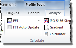
The Fourier transform of a profile is calculated by clicking on one of the Fourier functions in the Analyze > Calculate Panel in the Profile Tab group:
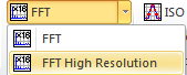
To achieve the highest accuracy it will be an advantage to apply the FFT High Resolution function (Requires the Extended Fourier or Calibration Module) , which means that the profile will be mean value padded so that it contains 16 times more elements before calculating its Fourier transform.
The Fourier curve will have its tool shown in the FFT Curve panel of the Chart Tools tab set.
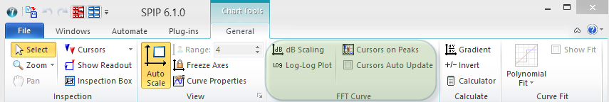
The function of the FFT Curve panel is described along with the other tab panels of the Chart Tools tab set.
Click dB Scaling to get the amplitude values of the Fourier graph shown in dB.
When the window contains an amplitude spectrum the fractal dimension can be evaluated from the Log Log function. The fractal dimension D is defined as
D = (6 + s)/2,
where s is the (negative) slope of the Log Log plot [John Russ]. The fractal dimension can also be calculated for all directions of an image as part of a roughness analysis.
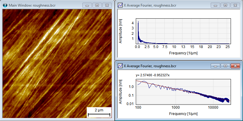
Log-Log example: From the image the Average X-Fourier is calculated and shown upper right. In the lower right curve the log-log presentation is shown and it is seen that its decay is highly linear. The best fit linear slope is -0.95, which results in an estimated fractal dimension of 2.5.
Click this function on and the four highest peaks will be detected and indicated by the cursors. When using this automated technique the peak positions will be calculated at sub-sample level by parabolic fits, so that the wavelength calculations shown in the graph will have a much higher accuracy. See example below.
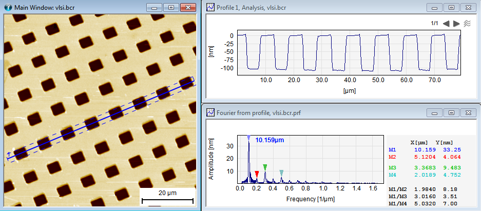
In the image a cross section line (in average mode) is put across the waffle structure and the corresponding profile is shown upper right. In the lower right the Fourier curve in shown. It has been calculated in high resolution mode and the four highest peaks have been detected. The very first and highest peak reflects the pitch distance which is approximately 10 um. The three other markers are associated with the 2nd, 3rd and 5th harmonic frequencies. The MX/M1 fields are used for testing the harmonic numbers; SPIP automatically divides the wavelength of the different cursors with the wavelength of curser M1. In this example, M1 points to the first harmonic, i.e., the pitch, M2, M3 and M4 are pointing to the 2nd, 3rd and 5th harmonics respectively, which is confirmed by the M1/M2, M1/M3, and M1/M4 fields. The higher harmonics can be used for getting a statically estimate of the pitch by multiplying the wavelength values by their harmonic numbers.
Note, that even though the x-axis is in reciprocal length unit the x marker values are shown in length unit for your convenience
Click this check mark to have the cursors update whenever the FFT curve is modified.