SPIP Classic Roughness Parameters for Images

The following describes the "SPIP Classic" surface roughness parameters implemented in SPIP™. All parameters recommended in the European BCR Project Scanning tunneling microscopy methods for roughness and micro hardness measurements are implemented and several other parameters applied by SPIP™ users is also included.

The table lists the roughness parameters by their symbol, name, corresponding 2D standard and unit.

Most parameters are general and valid for any M ´ N rectangular image. However, for some parameters related to the Fourier transform we assume that the image is quadrangular (M=N).

Before the calculation of the roughness parameters we recommend carrying out a slope correction by a 2nd or 3rd order polynomial plane fit. Note, also that roughness values depends strongly on measurement conditions especially scan range and sample density. It is therefore important to include the measurement conditions when reporting roughness data.

Some of the parameters depend on the definition of a local minimum and a local maximum. Here, a local minimum is defined as a pixel where all eight neighboring pixels are higher and a local maximum as a pixel where all eight neighboring pixels are lower.

As there are no pixels outside the borders of the image there are no local minimums or local maximums on the borders. Note that parameters based on local minimums and/or local maximums may be more sensitive to noise than other parameters.

The parameters are divided into four groups as described in the following.

Amplitude parameters

The amplitude properties are described by six parameters, which give information about the statistical average properties, the shape of the height distribution histogram and about extreme properties. All the parameters are based on two-dimensional standards that are extended to three dimensions.

The Roughness Average, Sa, is defined as:

Note, that since SPIP version 4.6 the mean value is not subtracted from the individual values, -which is according to the standards. You can still get the same results as before by selecting the roughness plane correction option to “Subtract Mean”.

The Root Mean Square (RMS) parameter Sq, is defined as:

Note, that since SPIP version 4.6 the mean value is not subtracted from the individual values, -which is according to the standards. You can still get the same results as before by selecting the roughness plane correction option to “Subtract Mean”.

The Surface Skewness, Ssk, describes the asymmetry of the height distribution histogram, and is defined as:

If Ssk = 0, a symmetric height distributions is indicated, for example, a Gaussian like. If Ssk < 0, it can be a bearing surface with holes and if Ssk > 0 it can be a flat surface with peaks. Values numerically greater than 1.0 may indicate extreme holes or peaks on the surface.
Note, that since SPIP version 4.6 the mean value is not subtracted from the individual values, -which is according to the standards. You can still get the same results as before by selecting the roughness plane correction option to “Subtract Mean”. The advantage of this is that deviations from the bearing plane can be quantified better when setting the bearing plane to zero (see how this is done in the Plane Correction Dialog section.)

The Surface Kurtosis, Sku, describes the “peakedness” of the surface topography, and is defined as:

For Gaussian height distributions Sku approaches 3.0 when increasing the number of pixels. Smaller values indicate broader height distributions and visa versa for values greater than 3.0.

Note, that since SPIP version 4.6 the mean value is not subtracted from the individual values, -which is according to the standards. You can still get the same results as before by selecting the roughness plane correction option to “Subtract Mean”.

The Peak-Peak Height, are denoted by three parameter names, Sz, St, Sy, according to ISO, ASME and reference [6]. They are defined as the height difference between the highest and lowest pixel in the image.

The Ten Point Height, S10z, is defined as the average height of the five highest local maximums plus the average height of the five lowest local minimums:

where zpi and zvi are the height of the ith highest local maximums and the ith lowest local minimums respectively. When there are less than five valid maximums or five valid minimums, the parameter is not defined.

Maximum Valley Depth Sv:, is defined as the largest valley depth value.

Maximum Peak Height Sp:, is defined as the largest peak height value.

Mean Height, S_mean is the mathematical mean height of all pixels.

Hybrid parameters

There are three hybrid parameters. These parameters reflect slope gradients and their calculations are based on local z-slopes.

The Mean Summit Curvature, Ssc, is the average of the principal curvature of the local maximums on the surface, and is defined as:

where dx and dy are the pixel separation distances.

The Root Mean Square Gradient, Sdq, is the RMS-value of the surface slope within the sampling area, and is defined as:

The Area Root Mean Square Slope, Sdq6, is similar to the Sdq but includes more neighbor pixels in the calculation of the slope for each pixel.

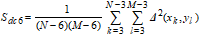
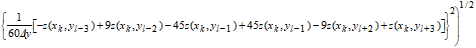
R9

The Surfaces Area Ratio, Sdr, expresses the increment of the interfacial surface area relative to the area of the projected (flat) x,y plane:

where Akl is defined as:

R11

For a totally flat surface, the surface area and the area of the xy plane are the same and Sdr = 0 %.

The Projected Area, S2A, expresses the area of the flat x,y plane as given in the denominator of R10.

The Surface Area, S3A, expresses the area of the surface area taking the z height into account as given in the numerator of R10.

Functional parameters for characterizing bearing and fluid retention properties

The functional parameters for characterizing bearing and fluid retention properties are described by six parameters. All six parameters are defined from the surface bearing area ratio curve shown in the figures below.

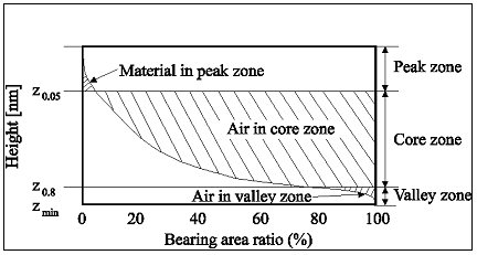
Figure 1: Bearing curve illustrating the calculation of Surface Bearing Index, Core Fluid Retention Index and Valley Fluid Retention Index

Abbott Curve

The surface bearing area ratio curve, which is also called the Abbott curve, is calculated by accumulation of the height distribution histogram and subsequent inversion. We divide both the histogram and the bearing curves into 500 intervals except for images having less than 5000 pixels where the intervals equal 10% of the total pixels.

The hybrid parameters can be described graphically by the above figure. Horizontal lines are drawn through the bearing area ratio curve at the ratio values 5% and 80%. These lines are marked Z0.05 and Z0.8 and the three zones created are called the peak, the core and the valley zone. Three parameters are calculated based on this figure-

The Surface Bearing Index, Sbi, is defined as:

where Z.05 is the height difference from the highest point and the surface height at 5% bearing area. For a Gaussian height distribution Sbi approaches 0.608 for increasing number of pixels. Large Sbi indicates a good bearing property. Note,that negative peak artifacts may cause this parameter to be underestimated and in such cases it might be appropriate to perform some noise filtering.

The Core Fluid Retention Index, Sci, is defined as:

where Vv(Zx), is the void area over the bearing area ratio curve and under the horizontal line Zx. For a Gaussian height distribution Sci approaches 1.56 for increasing number of pixels. Large values of Sci indicate that the void volume in the core zone is large. For all surfaces Sci is between 0 and 0.75 (Z0.05 -Z0.80) / Sq .

The Valley Fluid Retention Index, Svi, is defined as:

For a Gaussian height distribution Svi approaches 0.11 for increasing number of pixels. Large values of Svi indicate large void volumes in the valley zone. For all surfaces Svi is between 0 and 0.2 (Z0.80 -Zmin)/ Sq .

Parameters associated with the two-dimensional DIN 4776 standard are also calculated based on the bearing area ratio curve. First, draw the least mean squares line fitted to the 40% segment of the curve that results in the lowest decline, see figure below. Extend this line so that it cuts the vertical axes for 0% and 100% and draw horizontal lines at the intersection points. Then draw a straight line that starts at the intersection point between the bearing area ratio curve and the upper horizontal line, and end on the 0% axis, so that the area of this triangle is the same as the area between the horizontal line and the bearing area ratio curve. Using the same principle, draw a line between the lower horizontal line and the 100% axis.

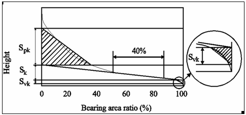
Figure 2: Bearing curve illustrating the calculation of Reduced Summit Height, Reduced Valley Height and Core Roughness Depth

The Reduced Summit Height, Spk, is the height of the upper left triangle.

The Core Roughness Depth, Sk, is the height difference between the intersection points of the found least mean square line.

The Reduced Valley Depth, Svk, is the height of the triangle drawn at 100%.

l-h% Height Intervals of Bearing Curve, Sdcl-h this is a set of parameters describing height differences between certain bearing area ratios; l and h denotes the lower and upper bearing area ratios of the interval. Sdcl is the height value at bearing area ratio at l % and Sdch is the bearing area ratio at h % and Sdcl-h denotes their height difference Sdcl - Sdch.

Currently SPIP calculates Sd0-5, Sdc5-10, Sdc10-50, Sdc50-95 and Sdc50-100.

Spatial parameters

The spatial properties are described by five parameters. These parameters are the density of summits, the texture direction, the dominating wavelength and two index parameters. The first parameter is calculated directly from the image, while the remaining are based on the Fourier spectrum. For these parameters we require the images to be quadratic.

The Density of Summits, Sds, is the number of local maximums per area:

Because, the parameter is sensitive to noisy peaks it should be interpreted carefully.

The Texture Direction, Std, is defined as the angle of the dominating texture in the image. For images consisting of parallel ridges, the texture direction is parallel to the direction of the ridges. If the ridges are perpendicular to the X-scan direction Std = 0. If the angle of the ridges is turned clockwise, the angle is positive and if the angle of the ridges is turned anti-clockwise, the angle becomes negative. This parameter is only meaningful if there is a dominating direction on the sample.

We calculate Std from the Fourier spectrum. The relative amplitudes for the different angles are found by summation of the amplitudes along M equiangularly separated radial lines, as shown in the figure below. The result is called the angular spectrum. Note that the Fourier spectrum is translated so that the DC component is at (M/2,M/2). The angle, a , of the i-th line is a = p/ M , where i=0, 1, .., M-1. The amplitude sum, A(a) , at a line with the angle, a , is defined as:

Figure 3: Fourier spectrum and the angular and radial spectra. a) Equidistant lines used for calculation of the angular spectrum shown in c).

b) Equidistant semicircles used for calculation of the radial spectrum shown in d).

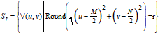
The angular spectrum is calculated by the following formula:

For non-integer values of and , the value of F(u(p),v(q)) is found by linear interpolation between the values of F(u(p),v(q)) in the 2x2 neighboring pixels. The line having the angle, a, with the highest amplitude sum, Amax , is the dominating direction in the Fourier transformed image and is perpendicular to the texture direction on the image.

Note that due to 1/f noise often a dominating direction parallel to the x-axis is found.

The Texture Direction Index, Stdi, is a measure of how dominant the dominating direction is, and is defined as the average amplitude sum divided by the amplitude sum of the dominating direction:

With this definition the Stdi value is always between 0 and 1. Surfaces with very dominant directions will have Stdi values close to zero and if the amplitude sum of all direction are similar, Stdi is close to 1.

The Radial Wavelength, Srw, is the dominating wavelength found in the radial spectrum. The radial spectrum is calculated by summation of amplitude values around M/(2 -1) equidistantly separated semicircles as indicated in sub figure (b). The radius measured in pixels of the semicircles, r, is in the range
r = 1, 2,.., M/(2 -1). The amplitude sum, b(r) , along a semicircle with the radius, r, is

The radial spectrum is calculated by the following formula:

Again the amplitude for non-integer values of
p=M/2 +r cos (i p/M) and q=M/2 +r sin (i p/M)
is calculated by linear interpolation between the values of F(u(p),v(q)) in the 2x2 neighboring pixels.

The Dominating Radial Wavelength, Srw, corresponds to the semicircle with radius, rmax , having the highest amplitude sum, bmax:

The Radial Wave Index, Srwi, is a measure of how dominant the dominating radial wavelength is, and is defined as the average amplitude sum divided by the amplitude sum of the dominating wavelength:

With this definition Srwi is always between 0 and 1. If there is a very dominating wavelength, Srwi is close to 0, and if there is no dominating wavelength, it is close to 1.

The Mean Half Wavelength, Shw, is based on the integrated radial spectrum :

Shw corresponds to the radius r0.5 where :

Having found r 0.5 , Shw is calculated this way:

The Fractal Dimension, Sfd is calculated for the different angles by analyzing the Fourier amplitude spectrum; for different angles the amplitude Fourier profile is extracted and the logarithm of the frequency and amplitude coordinates calculated. The fractal dimension, D, for each direction is then calculated as

where s is the (negative) slope of the log - log curves [John Russ]. The reported fractal dimension is the average for all directions.

The fractal dimension can also be evaluated from 2D Fourier spectra by application of the Log Log function. If the surface is fractal the Log Log graph should be highly linear, with at negative slope.

The Correlation Length parameters Scl20 and Scl37, are defined as the horizontal distance of the areal autocorrelation function that has the fastest decay to 20% and 37% respectively (37% is equivalent to 1/e).  For an anisotropic surface the correlation length is in the direction perpendicular to the surface lay.

The Texture Aspect Ratio Parameters, Str20 and Str37, are used to identify texture strength (uniformity of texture aspect).  It is defined as the ratio of the fastest to slowest decay to correlation 20% and 37% of the autocorrelation function respectively.  In principle, the texture aspect ratio has a value between 0 and 1.  For a surface with a dominant lay, the parameters will tend towards 0.00, whereas a spatially isotropic texture will result in a Str value of 1.00. If the autocorrelation for some direction does not decay below 20% or 37% the associated parameters will not be reported. This may be the case for image containing well organized linear structures.

Isotropic Area Power Spectral Density Function

One of the optional output graphs for Roughness Analysis is the Isotropic Area Power Spectral Density Function, which is based on the Area Power Spectral Density function defined below.

Area Power Spectral Density

This function can be shown by setting the "FFT Image Z Scale" to "Power Spectrum Density" in the Ribbon of the Fourier Image.

The Area Power Spectral Density function (APSD) for an image z(x,y) is defined [ASME B46.1-2002] as the square of the amplitude of the Fourier transform of the image normalized by the area size of a pixel:

where

The unit of APSD is m⁴

Calculation of the Isotropic Area Power Spectral Density Function

The Isotropic Area Power Spectral Density function is the APSD function integrated for all angles for given frequencies (inverse wavelength), i.e. it is the 2 Area Power Spectral Density Function reduced to 1D:

where

Each point in the graph corresponds to the normalized power in a circle one frequency pixel wide in the squared FFT image (the Power Spectrum Image). The unit of APSD is m⁴ and it is in SPIP displayed by the logarithmic values to make the weaker values more visible, see example below:

Example of an image where the Power Spectrum Density image and the Isotropic Area Power Spectral Density curve has been calculated.

SPIP offers the possibility to measure the RMS roughness within a frequency band by setting the cursors of the IAPSD curve at the desired band boundaries. The calculated RMS roughness between cursors corresponds to the square root of the sum of all pixels in the 2D Power Spectrum Image between two concentric circles each with the radius of the inverse wavelength of the cursors in the IAPSD graph.

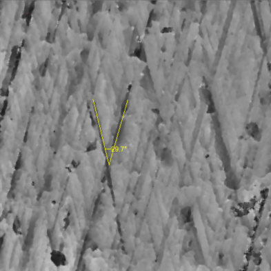
Cross Hatch Angle

The Cross Hatch Angle,Sch is the found angle of a cross hatch pattern typically created in seen in cylinder liners and created by a honing process used to ensure proper lubrication. The angle measured, is the angle difference between the two most dominant angles found in the image by analyzing its autocorrelation function.