
If you want to perform a lateral calibration with the highest accuracy the XY Linearity method is recommended. It will both calculate the best fitting unit cell along with linearity parameters for correcting the linearity and provide information about the average pixel location error useful for evaluating the uncertainty. In cases where the non-linearity is negligible you can save some processing time by using the "normal" unit cell detection method. For images which you just want to linearize without giving attention to the numerical correction parameters you might find it more convenient to use the XY Hysteresis correction method.
Please note that the calibration method requires that image contains a two dimensional uniform structure, such as the VLSI images shown in the below example.
Below is seen an example of part of the screen output after clicking XY Linearity:
Screen output after XY Linearity analysis. The image has the calculated lattice show by white lines and the local pixel dislocation is indicated by the red arrows. The size of the arrows indicates the relative magnitude of the errors and the dislocation direction. The errors are also visualized in the two scatter plots to the right; one showing the x-pixel error as function of the x-pixel position and the other similar for the y-direction. It is seen that non-linearities are very systematic and can be fitted very well to a third order polynomial. Therefore, it is also possible to calculate polynomial correction functions for linearizing the image.
In the above example everything was performed automatically and in the process a smaller image surrounding a found unit cell used as a template for finding the location (/dislocation) of similar structures. You can also define this template yourself by use of the Inspection Box and gain more control of the process. Selecting a large template will provide the most robust result but requires more computation time. Smaller templates can provide more information about the linearity close to the image borders. If you want SPIP to define a template you should make sure that the Inspection window is closed.
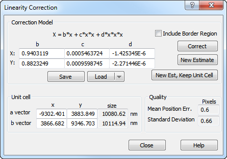
After a template has been selected (manually or automatically) SPIP starts the fine linearity analysis. If the unit cell has not been found earlier it will automatically be calculated by the Unit Cell Detection method. Then SPIP calculates the cross correlation function of the Inspection area and the entire image. The peaks of the cross correlation function are determined at subpixel level and determines the positions of all structures similar to the template shown in the Inspection window. It will compare the positions with those predicted from the unit cell data. The differences are described as linearity errors, which are further, minimized by minimizing the sum of square errors. The results are shown in the Linearity Correction Dialog , with more options and functional buttons:
:
The correction parameters are based on a third-order polynomial model of the scanning system. They describe how to resample the image. A more detailed description of the parameters is found in the reference guide. It is possible to enter your own values.
Sometimes it might be advantageous to omit the image borders as the position determinations are less accurate here. The disadvantage is that you will lose information obout the linearity close to the borders.
You can apply the correction parameters on the main image by clicking on the Correct button.
Recheck the linearity by clicking on New Estimate and you should observe that the correction parameters become more neutral, that the errors in the scatter diagram reduces to the sub-pixel level and that the Mean Position Error decreases. You may use this technique for checking the accuracy of SPIP in relation to the images you are analyzing.
When clicking on this button you will get a new estimation as above but without changing the current unit cell parameters. This gives you the possibility to see how sensitive the linearity analysis is to correct estimation of the unit cell.
The unit cell co-ordinates are found from a least error fit, except when the New Est, Keep Unit Cell button is used. In this case you may enter your own co-ordinates and observe how sensitive the analysis is to the unit cell co-ordinates.
The mean position error measure the combined X and Y dislocations. Regard also this as a quality measure for the combined
Linearity of the instrument
Uniformity of the surface structure
Accuracy of the image processing.
The calculated correction parameters can be stored and retrieved. To apply the correction parameters to a different image you can active this dialog directly from the ribbon bar: select Modify > Scaling and Correction > XY Linearization.
The extension of the linearity correction files is ".cpl"