![]() The height distribution histogram window is for image windows activate by clicking Analyze > Feature Analysis > Histogram and for profile windows by clicking Analyze > Calculate > Histogram.
The height distribution histogram window is for image windows activate by clicking Analyze > Feature Analysis > Histogram and for profile windows by clicking Analyze > Calculate > Histogram.
The histogram is an important analytical tool that provides important information about the height distribution and serves as an important tool for the Z-calibration algorithm.
It is a good idea to monitor the histogram while performing plane correction because the histogram is the best indicator for the flatness of the surface. Plane surfaces are characterized by high and narrow histogram peaks.
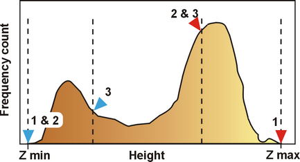
Below is seen an example of a histogram deduced from a z-calibration standard. The histogram exhibits two peaks from which the step height can be measured.
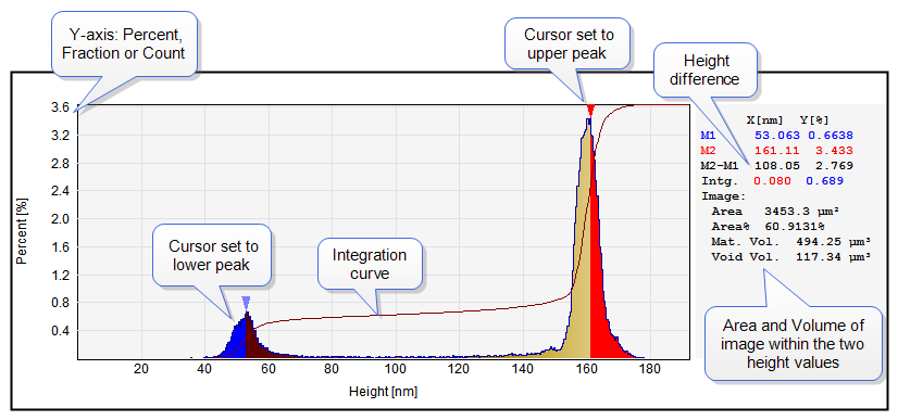
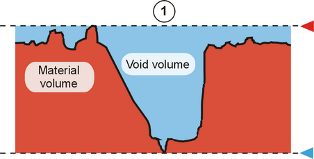
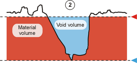
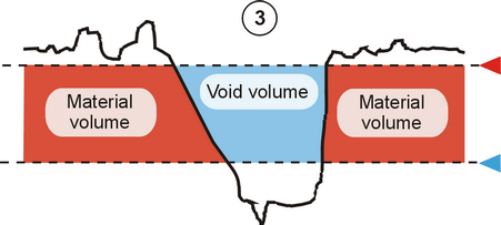
Based on the cursor positions you can also determine the area and volume for the range between the markers. There is provided two volume numbers: Material Volume (Mat. Vol.) and Void Volume (Void Vol.). All height values below the surface are considered as material while height values above the surface are considered as void. Thus it is possible to calculate the volumes between the height values given by the markers.
The figures below illustrate a situation where the void and material volumes are measured at different height ranges by moving the cursor position in the histogram:
|
|
|
 |
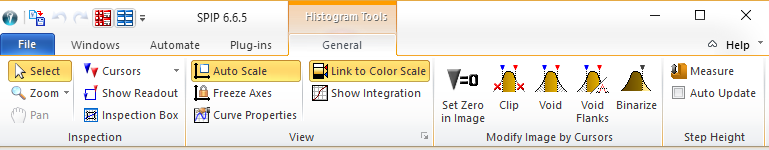
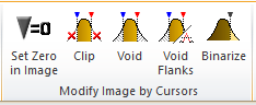
The different panels for the Histogram General tab is described below
This panel has the same functionality as the Inspection panel for profiles .
Click this button to activate the cursors, use the View Pane, or just press "C" on the keyboard. When pressed repeatable the number of cursor pairs will shift between 0, 1, and 2.
The cursors can be moved by mouse and for precise positioning by the arrow keys. The Up/Down arrow keys will move the cursor in the direction of a local summit, which is useful for finding local minimum or maximum points. When a cursor is positioned on a slope, it will be indicated by a tilt of the cursor. Summits are indicated by the cursors pointing straight downwards.
Setting Freeze Axes will freeze the y- and x-axes to their current range, such that a change of the histogram (for plane correcting the source image) will be reflected on the same scale. This serves as a good facility for comparing histograms on the same scale.
This will activate the Profile Property dialog where more parameters can be set. From the Property dialog it is possible to change the number of bins if the origin of the histogram is from an image or curve. For histograms based on particle analysis results the number of bins can be set in the Particle and Pore Output Setup dialog
Turn Link to Color Scale on to have the first cursor pair positions linked to the color clip markers of the "parent" image windows color scale.
Turn Show Integration On to display the Integration curve of the histogram. The difference between the integration values at the cursor positions reflect the relative surface area having height values between those marked with the cursor pair and will be indicated in the Area% numerical field.
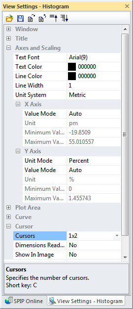
Different view options can be defined in the View Settings Pane belonging to the histogram. The view settings can be activated by clicking the Dialog Launcher button.
Offset the image such that the height value of the active cursor (last moved) is set to zero.
It is possible to use the first cursor pair for defining the lower and upper clipping values of the image and perform the clipping in the image by clicking this button.
This function work similar to the Clip to Markers, but instead of clipping it will define the pixels outside the z-boundary as void pixels.
This function works like the previous but in addition, it will also define pixels on the flanks of image features partly exceeding the threshold values defined by the cursor pair. This has shown to be useful in Particle & Pore Analysis for separating particles at different levels.
Below is seen an example on how the two Void functions work and differ.

Histogram Voiding Example: An image (in zoomed view) is seen with a cross-section line through a "bump" feature. Its corresponding profile is seen in upper right profile window. In the histogram window to the lower left the right red cursor is set to ~80 nm and thus defining this as the upper clip threshold value. The second right profile window shows the result after a "Void" operation and the lower right profile is the result of a "Void Flanks" operation and it is seen that the flanks now also have been voided.
This function will set all image pixels with values higher than where the active cursor (last moved) is positioned to 1 and all other pixels to zero. In this way a binary image is generated defined by the threshold given by the active cursor.
Click on Step Height to perform an automated step height measurement and calibration, see Z-calibration for further details. This function requires the Calibration Module to be included in the license.
Set Auto Update On to automate Z-Calibration measurements whenever the histogram is modified. This is for example practical when the histogram is linked to a profile of an image, in which case both the profile, the histogram and the Z-Calibration result is updated when moving the cross section line in the image.
Save As
The histogram data can be saved into an ASCII file or the STM-BCR file format or as graphical bitmap, jpeg or tiff file. The ASCII file contains the floating point x, y co-ordinate and can be imported by, for example, spreadsheet programs and the STM-BCR file can be read by SPIP.
Copy
The window can be copied to the clipboard by pressing CTRL+C and pasted into third party programs by pressing CTRL+V.
Duplicate
A duplicate of the window can be created by pressing CTRL+D or right clicking on Duplicate. Note, that the duplicate may only have single color bins because it is not connected to an image and its color scale.
To create a Normplot or "Normal Probability Plot" click on its button from the Histogram pull down menu:
The purpose of a normal probability plot is to graphically assess whether the data are normal distributed. If the data are normal distributed the plot will be linear. The x-axis represents the data values (typically height values) while the y-axis expresses the probability that a data value is equal or less some x-value (height value). The Y-axis is shown in percentage on a nonlinear scale (technically the y-axis corresponds to a linear axis with units of standard deviations). See example below:
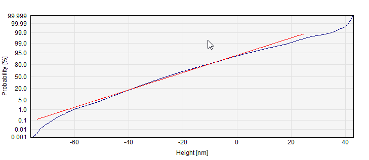
The red line in the chart corresponds to a normal distribution with the same mean and standard deviation as the image/profile data. Thus, deviations from the line expresses deviations from a normal distribution.
In the same way as for the histogram the markers are connected to the Color Clip markers and their functionality can be controlled from the Inspection panel.