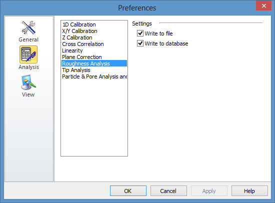
Roughness analysis for images works very similar to profile roughness analysis: The setup of desired parameters and charts is done from the Roughness Analysis Pane and the numerical results are shown in the Roughness Result Pane.
Currently the pre-processing of the image data offered by the Roughness Pane is restricted to plane correction . However, it is possible to perform other types of filtering using the Filter Module before performing the roughness calculation and it is also possible to have it included as at step in a Batch Processor sequence.
For Images the classic set of roughness parameters can be calculated and the numerical results shown in the Roughness Result pane. Depending on the options defined in the Preferences Dialog the results may also be written to files with the added extension .rgh or to the database of the ImageMet Explorer.

For convenience, the data are written in both a row and a column form in the .rgh output file. To combine roughness results from more files you may concatenate the files using a DOS command similar to this one:
"copy *.rgh results.argh"
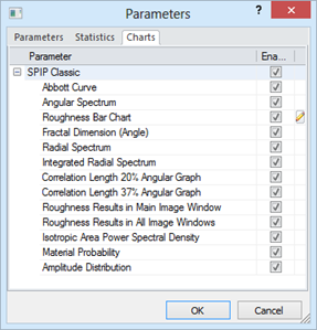
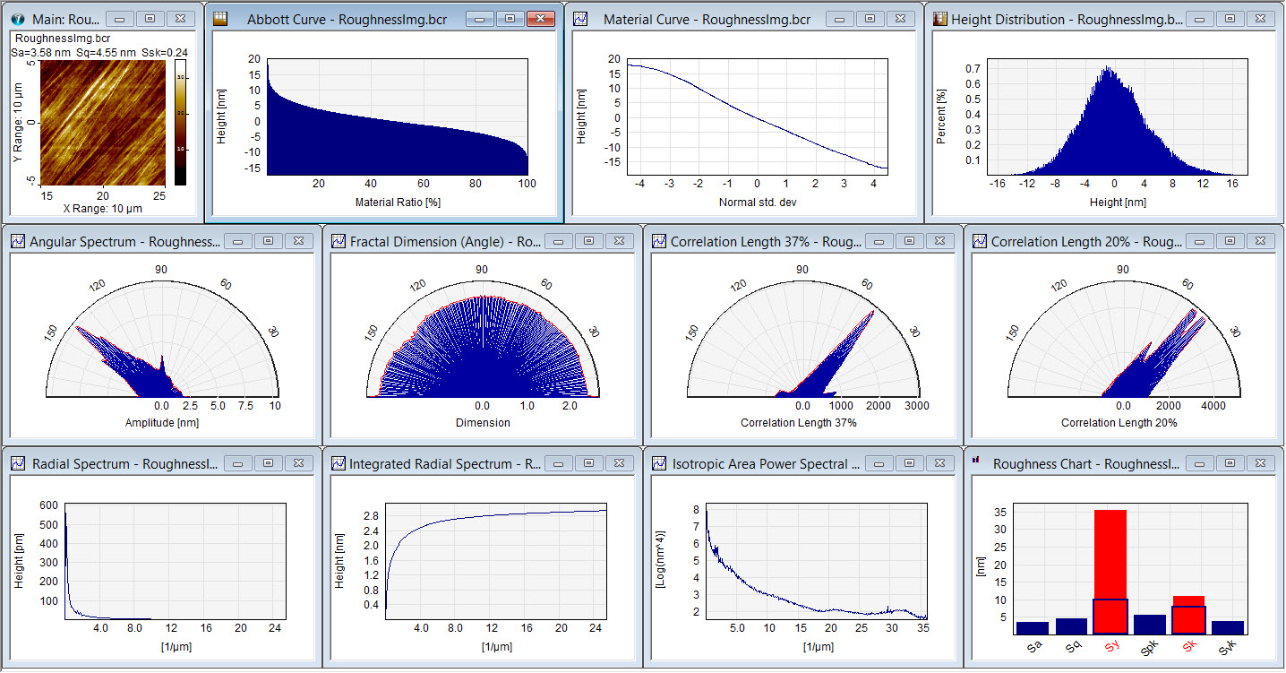
Several analytical graphs can be generated. These are selected from the Parameters Selection dialog (activated from the Roughness Analysis pane), see below. Examples of such graphs are the Material Ratio curve ( also called bearing or Abbott curve), the Angular Spectrum, the Radial Spectrum, the Integrated Radial Spectrum and the Fractal Dimensionand Area Power Spectral Density .
The angular spectrum and the fractal dimension are shown in Polar Plots (also called Rose Plots) with a value for all discrete angles between 0 and 180 degree.
Below is seen an example of a screen dump covering all the optional roughness charts:
One of the optional output charts for Roughness Analysis is the Isotropic Area Power Spectral Density Function described mathematically in the Reference Guide
This chart gives an intuitive overview of the distribution of wavelengths in the image, see example below:
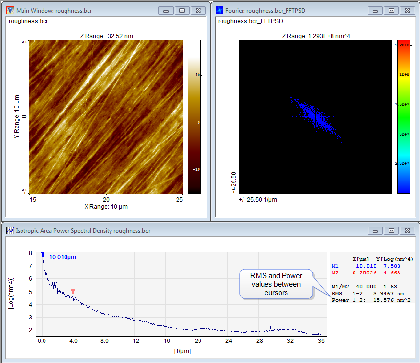
Example of an image where the Power Spectrum Density image and the Isotropic Area Power Spectral Density curve has been calculated.
SPIP offers the possibility to measure the RMS roughness within a frequency band by setting the cursors of the IAPSD curve at the desired band boundaries. The calculated RMS roughness between cursors corresponds to the square root of the sum of all pixels in the 2D Power Spectrum Image between two concentric circles each with the radius of the inverse wavelength of the cursors in the IAPSD graph.