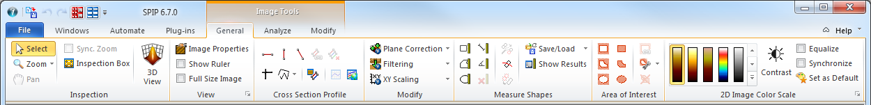
The following will describe the three ribbons dedicated to 2D Image Windows: The General, the Analyze and the Modify Ribbons.
The items of the General Ribbon will be described panel wise below:
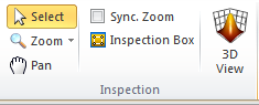
When the Select tool is highlighted none of the other tools are active. Clicking one of the drawing tools will highlight the active tool while the Select tool will be shown normally until the use of the drawing tool has finished. During drawing the mouse cursor will be seen as a shape reflecting the chosen tool instead of the normal mouse arrow.
You can zoom an image by:
To turn off zooming click Zoom > 100% or the Home key.
When zoomed, the lower right corner of the image will have a navigation area where you can see the entire image with an indication of the zoomed area.

When the panning tool is selected the zoom area can be panned either by dragging the entire image or by dragging the zoom box shown in the lower right navigation area.
The Inspection Box is used for closer inspection image details, where the image window in contrast to the zoom function are kept at the same scale, instead the interior of the box is shown in a "Inspection Window" with a caption showing the number of pixels contained. The Inspection Window is used in connection with a number of specialized analysis functions such as Correlation Averaging, XY Linearity Calibration for defining a template image.
Click this checkbox on to perform synchronized zoom, where all images of same size will be applied the same zoom factor and focus area. You can find an example where synchronized zoom was used in the description of the Analyze#8594;Compute Section
From the View Panel the Ruler/Scale bar and Color scale can be turned On/Off. The Image Property Dialog can be invoked and the View Settings can be activated from the dialog launcher button at the lower right.
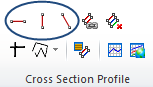
The three red cross-sections tools  are used for drawing cross-section lines in the image, horizontally, vertically and "free hand".
The Cross-section tools can be applied to all 2D image windows and will generate a cross-section profile window with corresponding cross section profile.
In some situations it can be convenient to move the line 1 pixel at a time by the arrow keys. The corresponding profile window will be updated simultaneously when changing the cross section line. To make straight horizontal or vertical line you can conveniently combine the mouse movement with the 'X' or 'Y' keys.
In some cases it might be desirable to reduce the noise content in the profile by averaging parallel cross-sections neighbors. This can be done interactively and described in the cross-section Profiling section.
 When Synchronized Profiling is set it is possible to create a profile for each image window having images of identical size and update them dynamically while moving or resizing the Line Marker in one of the image windows.
This technique can be valuable when dealing with image for the same physical area but showing different properties, for example height, friction, cantilever amplitude, phase, capacitance, magnetic force, etc. where it can be very practical to display profiles of the different images at the exact same cross-sections. This can be achieved by enabling Synchronized Profiling. When active a profile for each image window having images of identical size is dynamically updated while moving or resizing the Line Marker in one of the image windows.
Below is seen an example on how it can be applied for comparison of a filtered image with the original and the difference image.
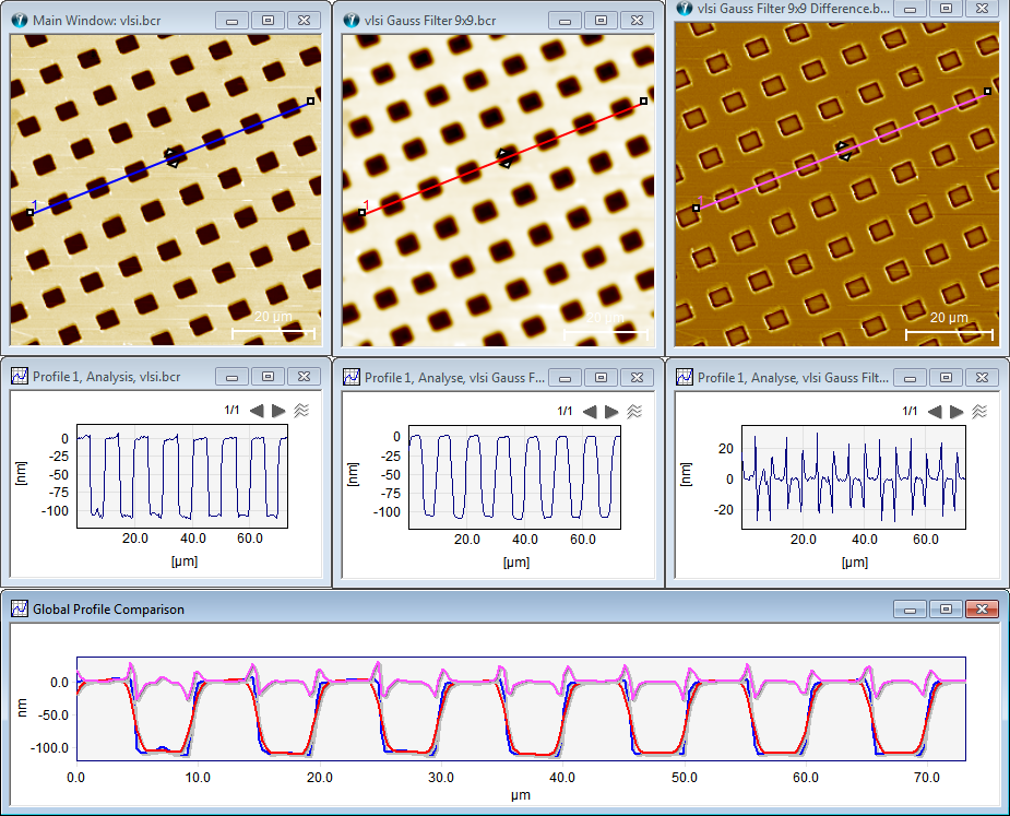
Synchronized Profiling example: Top left is the source image to its right is a filtered result after a Gauss smoothing filter. The right image is the difference image. All images have the cross-sections lines at the exact same locations. Below is seen the individual cross-section profiles and at the very bottom is the Global Profile Comparison window shown with all profiles together so that they can be compared more directly.
 Click this button to extract all x-profiles in the image into the same curve window.
 This function will force the profile window to appear. This may be useful when the Default Curve window is set to the Global Comparison Window in the Preferences dialog.
 This function will force the (one and only) Global Profile Comparison Window to appear. When creating a cross-section profile a copy of the profile will automatically be put into the Global Profile Comparison Window, even if it is hidden. Thus, this window is useful for comparing profiles from different sources. It can only show the profiles in comparison mode, but you can always perform measurements in the profile window related to a specific image window. An example on the usage of the Global Profile Comparison Window is shown in the Synchronize Profile example shown previously.
In the Preferences dialog you can define if you want to have the Global Profile Comparison Window to appear initially when defining a new cross-section.
 You can obtain a cross-section along a poly line by use of the Poly-line marker tool; the tool facilitates mainly three functions:
Drawing tool used for highlighting certain features in the image.
Profiling through image objects, which are not aligned on the same line.
Extraction of height profiles from Scanning Electron Microscope (SEM) Images.
When the Poly Line marker tool is activated each Left Mouse click will define a new point in the poly line. The Right Mouse button or the ESC key deactivates the drawing.
To clear the poly line, just select it and click the Delete button.
The positions of single points can be modified by the mouse after drawing has finished.
There is a pull down menu connected to the polyline tool where more specialized functions can be activated.
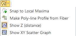
This function will try best as possible to define new points by following the highest values between the poly points. In combination with the Show XY-Scatter Graph function this is particularly useful for detailed analysis of SEM images showing surfaces structures in side view, i.e., the y-axis is associated with height.
This function creates the poly line cross section profile from the Fiber of a selected Polygon Measure Shape. The measure shape can for example be a DNA string and therefore this function can facilitate detailed topographic measurement of a DNA string.
The same function can be selected by right clicking on a "Polygon Measure Shape".
Below is seen an example of an poly-line profile extracted from a calculated Fiber of a detected shape:


When the Show Z(Dist) is active the profile through the defined line segments is calculated and shown as a graph.
A scatter diagram showing the path of the polyline can be created by this function and the graph can be used for performing different types of measurements.
![]() By use of the Cross Hair marker you can obtain horizontal and vertical cross-section profiles simultaneously. These profiles will be shown in their own profile windows in Analysis View only.
By use of the Cross Hair marker you can obtain horizontal and vertical cross-section profiles simultaneously. These profiles will be shown in their own profile windows in Analysis View only.
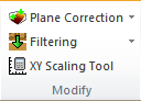
The Modify Panel contains frequently used modification tools for Plane Correction (flattening) Filtering and a button for activation of the XY Scaling Pane.
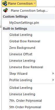
Filtering and plane correction can be applied directly without opening the corresponding dialogs by selecting predefined Built-in and custom made setting files from the pull down menus as shown below for plane correction.
The Plane Correction and Filtering functions can also be accessed from the Modify tab group.
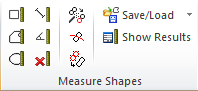
The Measure Shape tools allow the user to make a wide range of measurements interactively by drawing the available Shapes in an image. The results are shown in a spreadsheet like pane (the Shape Measurements pane) in histograms, in scatter plots or directly in the image. The tools are described in more detail in the Measure Shape Tools topic.
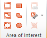
The Area of Interest (AOI) drawing tools are used for including or excluding certain areas from analysis and modification, or to define pixels as void pixels. The tools are described more detailed in Area of Interest Tools
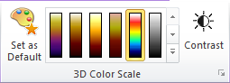
The Color Scale Panel facilitates an easy selection of predefined built-in or custom made color scales.
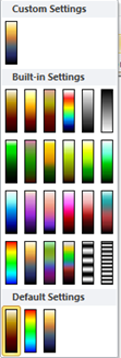
By clicking on the "More" button  all predefined color scales will be listed and made available for selection:
You can select the Color Equalize mode for enhancing the image contrast or Synchronize the colors such that all open image windows will be using the same color scale.
To have all shown images to use the selected color bar click the Synchronize check box On.
The dialog launcher button  will activate the . The Colors and Presentation section covers the features related to the color scaling more detailed.
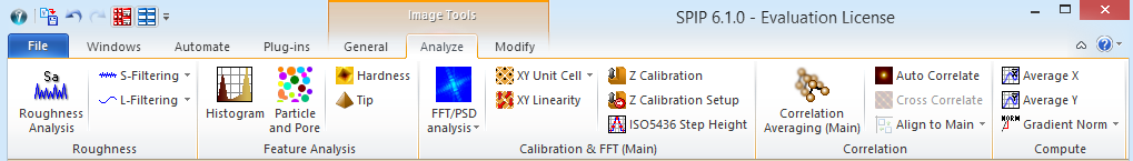
The Analyze Ribbon contains all the tools for analyzing images. These functions are described panel wise below:
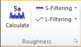
The Calculate button will calculate the roughness parameters and graphs defined in the preferences dialog, which can be opened by the dialog launch button
You may preprocess by standard filters. The S-Filters are used for filtering short wave lengths (typically noise) in the image by applying an ISO 16610 Gaussian S Filter according to the ISO 25178-2 standard. The L-Filters are used for filtering the long wave lengths (background waviness and slopes) in the image by applying an ISO 16610 Gaussian L Filter according to the ISO 25178-2 standard.
You can learn more about roughness in the Roughness Analysis section.
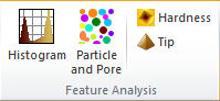
The Feature Analysis panel contains tools for extracting features, quantitative and graphically.
For more detailed description see the following sections Histogram, Particle and Pore Analysis, Hardness Analysis and Tip Characterization.
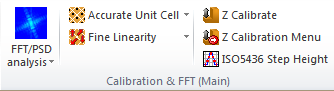
This panel contains tools for calibration and Fourier Analysis.
The FFT/PSD Button will perform a Fast Fourier Transformation and show the result in the Fourier Window. The ribbon tab from the Fourier Window will show more dedicated tools and the Fourier result can be scaled in different ways, one scale option is the Power Spectrum Density (PSD).
To perform a lateral calibration you will need an image with a well-defined lattice structure. The Unit Cell detection functions and the Fine Linearity function can then calculate the unit cell and provide calibration values. The Fine Linearity function will be the most accurate and provide the most detailed information but it is also the most time consuming.
You can learn more about the different tools in their respective sections: Fourier Analysis, Unit Cell Detection, Linearity Analysis, Z Calibration and Z Calibration based on ISO5436 Profile Analysis
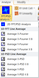
The FFT Line Average Functions will calculate Fourier amplitude spectra for each X line or Y column and the calculate the average amplitude spectrum. This way correlated structures may become visible so that interactive measurements can be performed.
When the "X 8" resolution functions are used the individual profiles will enlarged eight times by mean value padding so that Fourier peaks can be found with 8 times higher resolution.
The PSD Line Average Functions will calculate PSD spectra for each X line or Y column and then calculate the average PSD spectrum.
Here, each Z value is calculated as the power value normalized with the are size of each element
 ,
,
where P(u) is the Power value for the Fourier index u and Range is the physical range of the profiles.
Click the XY Unit Cell button or Fast Unit Cell to get a calculation of the unit cell (if applicable). An example of a detected unit cell is seen in the Fourier Analysis section.
Click this button to perform a Linearity Analysis
Click this button to perform a Z Calibration
Click this button to prepare a z-calibration and open the Z Calibration Dialog
Click this button to perform a Z Calibration based on ISO5436 Profile Analysis

The correlation Panel contains tools for activation of correlation functions and alignment of images based on correlation analysis.
The functions are described more detailed in the following sections: Correlation Averaging, Auto Correlation, Cross Correlation and Align to Main.
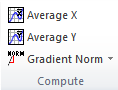
The Compute Panel contains function for calculation of X-, Y- Average Profiles and gradient images.
This function will calculate the average x-profiles and show the result in a Single Curve window (without comparison view mode)
This function will calculate the average y-profiles and show the result in a Single Curve window (without comparison view mode)
The Gradient pull down menu provides the following functions for calculation of gradient dependent images:
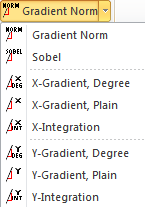
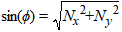
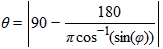
The Gradient Norm describes the angle of the local normal vector minus 90 degree. Thus for a flat surface the values will be zero degree. For high slopes the angle may approach 90 degree.
The way the angle θ of the normal vector N is calculated in SPIP is as follows:
For point x,y we calculate four normal vectors based on four triangles around the point P0,0:
P 0, 0 = (x, y, z(x,y))
P 1, 0 = (x+1, y, z(x+1,y))
P 0, 1 = (x, y+1, z(x,y+1))
P-1, 0 = (x-1, y, z(x-1,y))
P 0,-1 = (x, y-1, z(x,y-1))
N1 = Normal vector of Triangle P0,0, P1,0, P0,1,
N2 = Normal vector of Triangle P0,0, P0,-1, P-1,0,
N3 = Normal vector of Triangle P0,0, P-1,0, P0,1
N4 = Normal vector of Triangle P0,0, P0,-1, P1,0,
Na = (N1+N2+N3+N4)/4
N = Na/│Na│
Sobel is an edge enhancement filter described in the Edge Enhancement Filter section
The X-Gradient is a simple calculation of the dz/dx values. Thus it will highlight x-directional structures. The gradient values can be expressed by their direct numbers or the corresponding angles.
The X-Gradient, Degree is calculated as (180/Pi)*atan(dz/dx) using the physical units in z and x dimensions.Relative flat surfaces will have angle values close to zero.
The X-Integration function will perform an integration in the x-direction, which except for the general height level will be the inverse function of the X-Gradient.
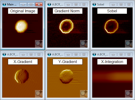
Gradient image example. The images are created by using the gradient tools described above. Synchronized zoom was used for obtaining these images where it is zoomed into the same feature.
As the name indicates the Modify Ribbon contains tool for modifying images. This can for example be noise filtering or filtering for enhancing images structures.

The Plane Correction panel includes tools for background removal (also called flattening or slope correction) such that real surface structure becomes more apparent. It includes also line wise correction methods which are good for images that has been created by raster scan techniques and where there can be a z-drift between the individual scan lines.
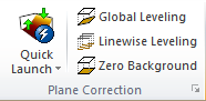
You can use the Plane Correction Quick Launch to select and apply built-in or you own saved Plane Correction Settings or open the Plane Correction Dialog where you have access to all settings.
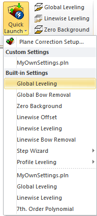
The Global and Linewise Leveling serves as quick access to plane correction methods that will work relatively well for most images. The Zero Background tool will set the background z-value to zero where the background value is defined as the most frequent z-value found by histogram analysis.
The Plane Correction dialog, which may also be opened by the Dialog Launcher , and correction techniques are described in the chapter Plane Correction and Flattening.
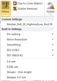
Use the Quick Launch to select and apply built-in filters or your own saved filters.
You can use the clip to Color Markers tool to clip z-values outside the boundary marked by the right clip markers on the Color Scale.
The Outlier Removal button will open the Filter Outlier Objects dialog, which will provide more advanced tool for filtering outliers.
![]()
The Transformation panel contains tools for rotation, flip (mirror) and resizing the number of pixels.
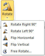
Use these two functions for 90° rotation.
These functions will flip (mirror) the image horizontally or vertically.
For Free Rotation click this button, which will activate the Rotation dialog with more specialized functions.
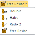
The Double key will increase the number of pixels by 2x2 using linear interpolation. This may be useful for increasing accuracy in various measurements and analysis.
The Halve key will decrease the number of pixels by 2x2. This may be useful for decreasing computations time in various measurements and analysis.
This function increases the number of x,y pixels to the nearest radix two numbers, which often increases the Fast Fourier transform calculation
Clicking Free Resize will activate the Property dialog of the image where the number of pixels can be set freely.
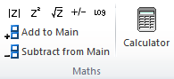
In the Math Panel it is possible to perform different types of mathematical operation on images, such as subtracting two images from each other for comparison reasons. The Square Root and Log function will generate void pixels in case of negative values.
The calculator button will open the Image Calculator Pane where you can combine mathematical expressions for calculating new images.
Click the Calculator button to activate the Calculator pane where calculations with input from one or more images can be performed and output the results in new image windows.

The Void Pixels Panel let you handle void pixels, which has not been measured or has been defined as void for other reasons, such as extreme values.
Some Images may contain "void pixels", which are pixels that could not be measured by the instrument. This is often true for interference microscope images, which need a proper reflectance in order to measure the height values. This may also be true for objects with holes for examples rings. Void pixels can be handled as invisible when drawing in 2D or 3D or they can be shown by other inserted values. For visualization purposes you may want to enhance a certain feature making its surroundings invisible by turning it into void pixels (see 3D example). Likewise void pixels are excluded from various modifications and analysis.
The number of void pixels contained in the image is shown in the Image Property Dialog.
You may also find it convenient to use the View Settings#8594; Image Section for showing the void pixel areas as invisible (in which case the background color of the window will be used) or visible meaning that the underlying pixel values will be shown.
When having void pixels it is possible to Fill in the specific statistical values shown below or Fill in the values underneath the void pixel mask and make them valid pixels.
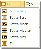
This function will clear the void mask and turn void pixels into valid pixels by using the underlying pixel values.
The Mask Main works on the Main Image Window, such that all pixels in the active image having a value outside the z-range, defined by the right color clip markers, will cause the corresponding pixel in the main image to be defined as void pixel.
Use this function to mark pixel with values outside the Color Clip Markers or the corresponding markers in the Histogram window as Void pixels. This may be a useful technique for eliminating the influence from outlier values.
Use this function to mark areas outside marked AOI's as Void pixels. The same function is also available from the AOI context menu.
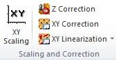
The Scaling and Correction Group is used for correcting the X, Y, Z scaling of an image. You will need to enter scaling parameters, which you may have obtained from the x,y calibration function or the z-calibration functions by use of reference samples.
Click the XY Scaling button to activate the XY Scaling Tool pane. This pane is primarily use for images where the physical x,y dimensions are not embedded in the file, but where you can take advantage of a scaling bar overlaid in the image. This can typically be a SEM image. The tool will work with the same correction factor for both the X and Y dimensions. You can learn more about how to use the tool in the XY Scaling Tool section.
Click this button to activate the Z-Calibration dialog, which enables you to correct the z-values by a correction factor or to initiate a calculation of a step height and corresponding correction factor.
This function will activate the Unit Cell and Calibration Results dialog, which facilitates independent correction parameters for the X and Y dimensions and in addition you can also enter and skewness parameter caused by x,y coupling or drift during a raster scan. The tools also provide an interactive facility for defining a unit cell such that correction parameters can be calculated when the true reference parameters are known.
Click XY Linearization to activate the Linearity Correction dialog, where 3rd order correction parameters for both X and Y can be inserted or recalculated such that lateral linearization errors can be corrected.
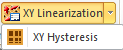
This button is a pull down menu item of the XY Linearization. It will invoke a hysteresis correction based on independent 2nd order for X and Y.